Center for Earth Observing and Spatial Research


El Niño Update for September 2026

El Niño events occur every two to seven years, and they are driven by feedback between ocean currents and the circulation of the atmosphere over the tropical Pacific Ocean. Variation in ocean temperature and wind patterns drives variation in the rain and snow that falls over the tropical Pacific and elsewhere in the world. Many forecasts have been issued for the El Niño that started in the summer of 2026, and past El Niños have been extensively discussed during the months leading up to this one. One way that NASA contributes to the conversation is to provide, in near real time, estimates of how much precipitation falls over oceans and continents. GMU’s CEOSR team assists NASA with evaluating these precipitation estimates and with evaluating new versions of the precipitation-estimating algorithm before they becomes operational.

A few hours after September ended, NASA provided initial, near real-time estimates of July–September precipitation totals around the world. These three-month totals deviated significantly from seasonal averages in many places. For example, part of India this summer experienced its worst drought since 2015, another year when a strong El Niño was ramping up. Most strong El Niños start in spring or summer and last until the following spring, and so they are named after these two years, such as 2026–27.

Not every precipitation anomaly that occurs during an El Niño is caused by the El Niño, and it will take years of study for scientists to fully understand the story of the 2026–27 El Niño. Nonetheless, it is an important first step to measure precipitation globally and to identify the ways that, during the 2026–27 El Niño, precipitation differs from the long-term average. Such research can contribute to mitigating the societal harm that the current or a future El Niño could cause.

Three-Month Precipitation Totals from NASA’s IMERG

The simplest way to evaluate the precipitation that fell this July through September is to compare it to the long-term average for this time of year. NASA monitors rainfall and snowfall in near real time using IMERG, the agency’s data-processing algorithm that combines observations from all available satellites that observe the Earth at microwave or infrared frequencies. IMERG stands for Integrated Multi-satellitE Retrievals for the Global Precipitation Measurement (GPM) Mission. IMERG estimates global precipitation every 30 minutes at approximately 11-kilometer resolution (0.1°⨯0.1° in latitude and longitude). IMERG estimates are available from January 1998 onward.
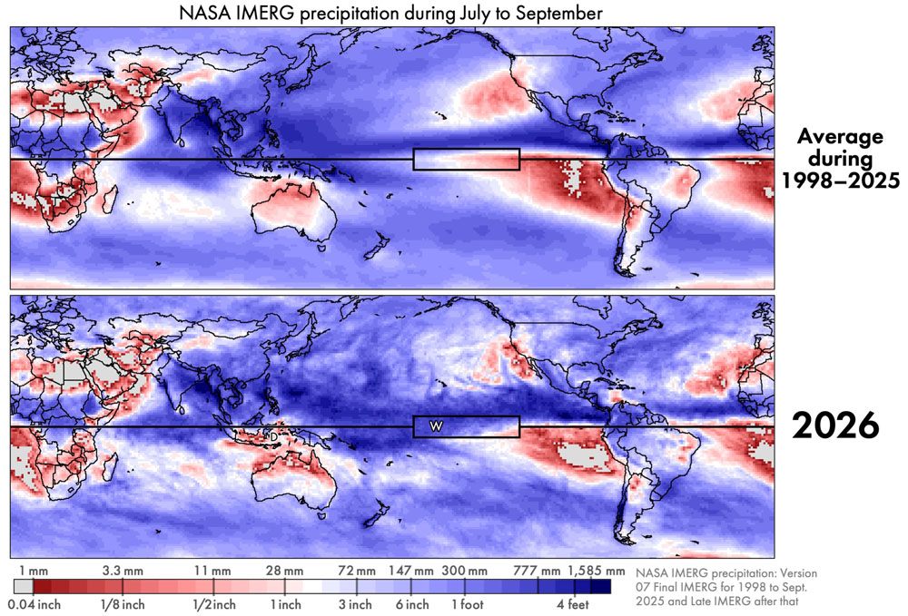
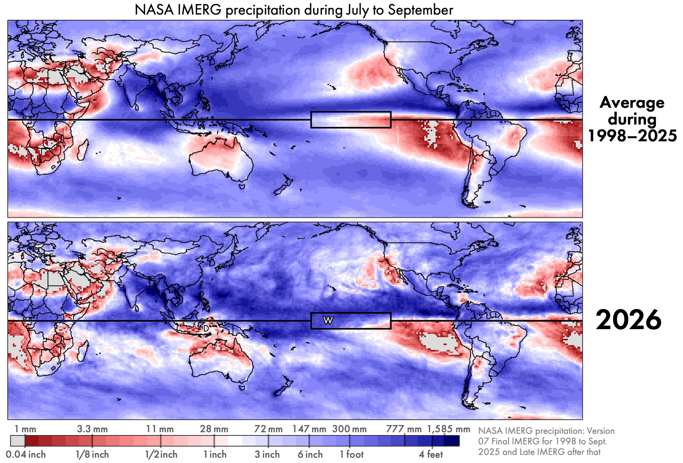
Figure 1. IMERG precipitation accumulation for July through September either averaging over 1998–2025 (top) or just during 2026 (bottom) [High-res image]

El Niño changes some aspects of global precipitation but is powerless to change other aspects of it. Regardless of the state of El Niño or other atmospheric oscillations, the approximate location of Earth’s wettest and driest places remains about the same. And the range of annual accumulation is huge: about a factor of 100. The annual accumulation of rain and snow is under 1 inch in some places and over a 100 inches elsewhere (<25.4 mm vs. >2,540 mm). For July through September, Figure 1 shows deserts in light gray and the places with the most precipitation in dark blue. In these totals, any snowfall is represented by the depth it would have if it were melted.

Throughout the year, frequent storms near the Equator cause this region’s rainfall accumulation to be among the largest on Earth. In the subtropics, there are several permanent patches of extreme desert over land or ocean. Despite the persistence of these large-scale precipitation zones, their boundaries do shift a bit throughout the year and from year to year. In Figure 1, the Equator is depicted by the black horizontal line. The box along the Equator is the Niño 3.4 region where sea surface temperature is monitored to determine when an El Niño event is occurring.

Unusual aspects of precipitation during 2026 can be seen in Figure 1, but not very clearly. Near the Equator, the three-month period of July–September 2026 saw more precipitation than average in the Central Pacific and less precipitation than average in the East Pacific. It is easier to see such differences if they are explicitly plotted.

Percent Difference and Absolute Difference

Examining two kinds of differences can help interpret the rainfall data: absolute difference and percent difference. An absolute difference is calculated by subtracting a reference values from current conditions, and it has units of millimeters of precipitation accumulation. Alternatively, one can display the percent difference between current and reference values. For the data examined here, the current conditions are the three-month accumulation from IMERG during July–September 2026 and the reference value is the average July–September accumulation from IMERG during 1998–2025. The difference between current conditions and the long-term average is often called an anomaly by atmospheric scientists. The use of the term anomaly does not mean that the observed difference is necessarily surprising or dangerous.

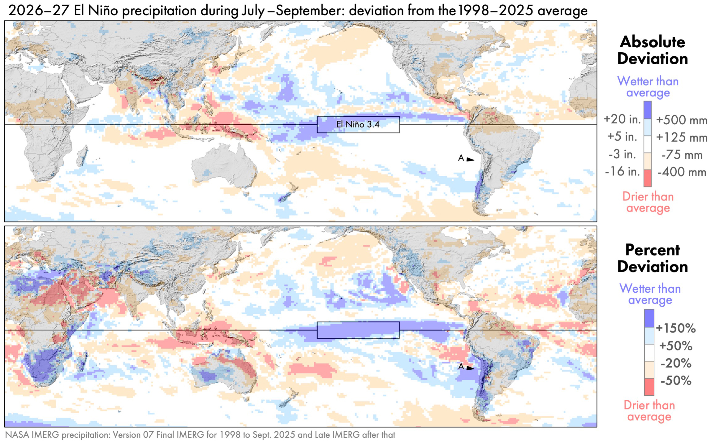
Figure 2. IMERG precipitation anomalies for July–September 2026: absolute difference (top) and percent difference (bottom) [High-res image]

In absolute terms, the two largest anomalies during July–September 2026 occurred near the Equator over the Pacific Ocean. Precipitation was 500 millimeter (20 inches) greater than average in part of the Central Pacific and 400 millimeters (16 inches) less than average in part of the Western Pacific. These features are dark blue and dark red, respectively, in the top panel of Figure 2.

If one looks only at absolute difference, then one will miss most of the precipitation anomalies that occur in arid regions. For example, consider the west coast of South America, and specifically Chile’s Atacama Desert. This desert is identified by point A in the bottom panel of Figure 2. The absolute anomaly here is near zero (white in the top panel). Yet, a large relative increase in precipitation is seen in the percent-difference map (dark blue in the bottom panel).

Illustrating this point, the Chile meteorological agency reported that a particular rain gauge in the Atacama Desert receives an average of 4 mm (0.16 inches) per year of precipitation, but it received much more, 14.8 mm (0.58 inches), in August 2026. This gauge (#230001) is located along the west coast of South America. Consistent with this rain-gauge data, the satellite-based IMERG estimate was that the July–September 2026 rainfall total at this location was more than 150% above the long-term average.

It can be difficult for a satellite-based dataset to provide accurate estimates of precipitation in an arid location because there is so little precipitation to see there. One way to increase confidence in near real-time IMERG estimates is to compare them to an independent dataset that is also available in near real time. Within a few days of a month ending, the German meteorological service creates the GPCC First Guess dataset for that month, based on the limited number of rain gauges around the world whose observations are published in time to be included.

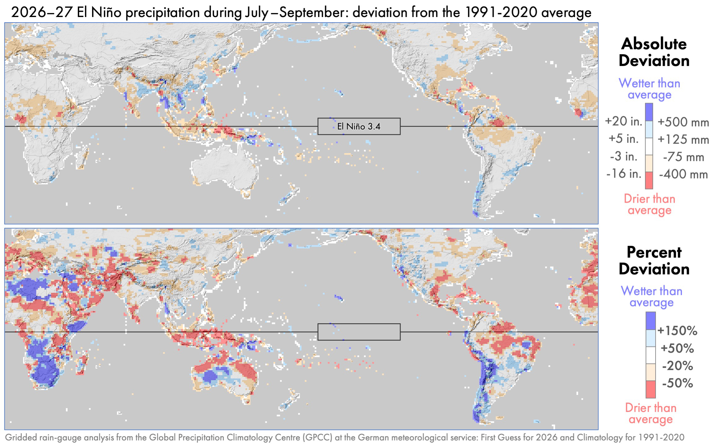
Figure 3. Precipitation anomalies for the same period as Figure 2 except using GPCC rain-gauge estimates rather than IMERG satellite estimates [High-res image]

One would expect global precipitation patterns to differ somewhat depending on whether they are based on observations from rain gauges or polar-orbiting satellites. Rain gauges continuously collect information throughout the day, but are separated by large distances. Polar-orbiting satellites fly over a location for just one instant, but they cover a region with a dense set of observations when an overflight does occur. Despite the different strengths and weaknesses of these instruments, gauge and satellite datasets show remarkably similar large-scale features in this case. During July–September 2026, both datasets show similar precipitation anomalies, comparing Figures 2 and 3. The two datasets generally agree on the sign of the large-scale precipitation anomalies on each continent and their approximately location.

Rain Over the Atacama Desert

According to IMERG, the Atacama Desert in northern Chile received precipitation during July–September 2026 that was 150% above the average amount for this time of year. In other words, 2.5 times normal precipitation fell: 100% of the normal amount plus an extra amount equal to 150% of the normal amount.

While the 2026–27 El Niño brought heavy rain to the Atacama Desert, this pattern was not following during the four strongest El Niños during 1998–2025. These four El Niños occurred in 2002–03, 2009–10, 2015–16, and 2023–24. Whether an El Niño is categorized as strong or not can depend on whether one is looking at the ONI or RONI index to measure it.

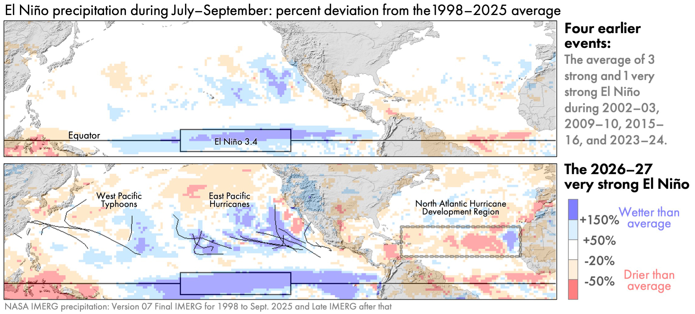
Figure 4. July–September precipitation anomaly during typical El Niño years (top) or during the El Niño that started in the summer of 2026 (bottom) [High-res image]

The bottom panel of Figure 4 shows that the early months of the 2026–27 El Niño had far more precipitation over the Atacama Desert that was typical during prior El Niños (top panel of Figure 4). Much of this rain fell on a single day, namely August 18, 2026. The figure below shows a satellite overflight of the storm that brought this rain. The data was collected by the passive-microwave instrument on the Core Observatory satellite of NASA’s Global Precipitation Measurement (GPM) Mission. The instrument is called the GPM Microwave Imager, or GMI for short. Microwave radiometers like GMI have the advantage of seeing into clouds to provide X-ray-like 2D images. In contrast, satellite instruments observing infrared radiation can only gather information about the height of cloud tops, which is a measurement that is only loosely tied to a storm’s ability to produce heavy rain at the Earth’s surface.

Figure 5 (below) is a false-color image generated using three frequencies of radiation measured by GMI, each one controlling the amount of red, green, or blue in the image. This visualization technique was first proposed by Negri et al. (1987). In the false-color image, GMI data over ocean is green-blue where the air column is dry and dark blue where the air column holds more water vapor. Over ocean, low clouds are black and high clouds are light gray. Cloud-free land is dark green-brown. The figure shows six GMI overflights, with the gaps between them filled with infrared satellite observations of cloud-top height.

Figure 5. GMI observations of storms bringing rain to Chile on August 18, 2026 [High-res image]

Labeled L in the figure, a cutoff low on August 18, 2026, was pulling humid tropical air south to fuel the precipitation over the Atacama Desert in northern Chile. Cutoff lows are fairly common off the west coast of South America, but this one formed a bit further north than usual (Fuenzalida et al. 2005). Cutoff lows contribute to the formation of a significant number of the rare, heavy precipitation events in several arid regions around the world (de Vries et al. 2024). Cutoff lows can be identified using the archive of upper-air charts at the University of Wyoming.

Also on August 18, an atmospheric river was bringing humid tropical air south to the forests of central Chile. An atmospheric river is a channel of fast-moving low-altitude air (a low-level jet) carrying water vapor to mid-latitudes. Most atmospheric rivers flow across the front edge of an advancing cold front (Dacre and Clark 2025, Figure 3). Most atmospheric rivers than usual reach the southwestern coast of South America during El Niño years (Gibson et al. 2026, Figure 9).

Hurricanes and Typhoons

During July–September of almost every year, tropical cyclones form in three places: the North Atlantic, Northeast Pacific, and Northwest Pacific. These storms are called typhoons in the Northwest Pacific and hurricanes elsewhere.

Associated with the very late start to the 2026 Atlantic hurricane season was below-average precipitation in a large portion of the North Atlantic during this time. It was very unusual that 2026 saw no hurricanes in the North Atlantic during July–September. According to NOAA’s records, 2026 was the first time in over a century that this happened.

During an average year, the Atlantic has seven hurricanes during the season that officially runs from June through November. There were two to four Atlantic hurricanes during three prior very strong El Niños, which were in 1982–83, 1997–98, and 2015–16. Another measure of hurricane and tropical storm activity is called ACE, which stands for Accumulated Cyclone Energy (NOAA 2026, footnote c). By the end of September 2026, the Atlantic value for ACE had reached only 11% of the value that typically occurs by the end of the Atlantic hurricane season. It was not until October 8, 2026, that Hurricane Isaias became the first Atlantic hurricane of the year.

The figure below shows the tracks of tropical cyclones as black lines using data from the National Hurricane center east of the International Date Line and from the Natyphoon website as compiled by Wikipedia west of the International Date Line.
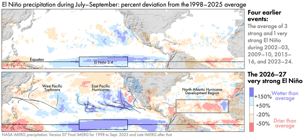
Figure 6. July–September precipitation anomaly over Northern Hemisphere oceans during typical El Niño years (top) vs. during 2026 (bottom) [High-res image]

In contrast to the North Atlantic, there was above-average hurricane activity in the East Pacific during July–September 2026. These hurricanes contributed to above-average rainfall there. An average year sees eight hurricanes in the East Pacific, and there was one more than that during July–September 2026. More importantly, the ACE index of hurricane activity, as of the end of September 2026, was almost double the average value at the end of an East Pacific hurricane season (95% above normal).

Despite the limited coverage of a single satellite instrument, a day’s worth of observations can sometimes hint at the large-scale state of the atmosphere. For example, the GMI radiometer collected observations on September 4, 2026, that hinted at the active nature of this year’s East Pacific hurricane season. GMI observed three East Pacific hurricanes that day, a rare occurrence in the instrument’s data archive.

Figure 7. GMI observations of three hurricanes in the East Pacific on September 4, 2026 [High-res image]

Global Comparisons to Other El Niños

During July–September 2026, the precipitation excesses and deficits were larger than those during the early months of the four prior El Niños that were classified as moderate to very strong. The global maps below reveal that, during these three months of 2026, there were several yet-to-be-discussed regions with precipitation anomalies that were large even by El Niño standards.

Figure 8. The July–September global precipitation anomaly for four prior strong El Niños and the analogous precipitation anomaly for the 2026–27 El Niño [High-res image]

For the most part, the location of precipitation anomalies in 2026 are similar to those in prior El Niños. It’s just that their magnitude and geographic extent in 2026 are greater than during prior events.

Global maps of precipitation anomalies contain many details, and it can be difficult to determine which of these details are a distraction and which are important. To emphasize important details, researchers create schematic diagrams.

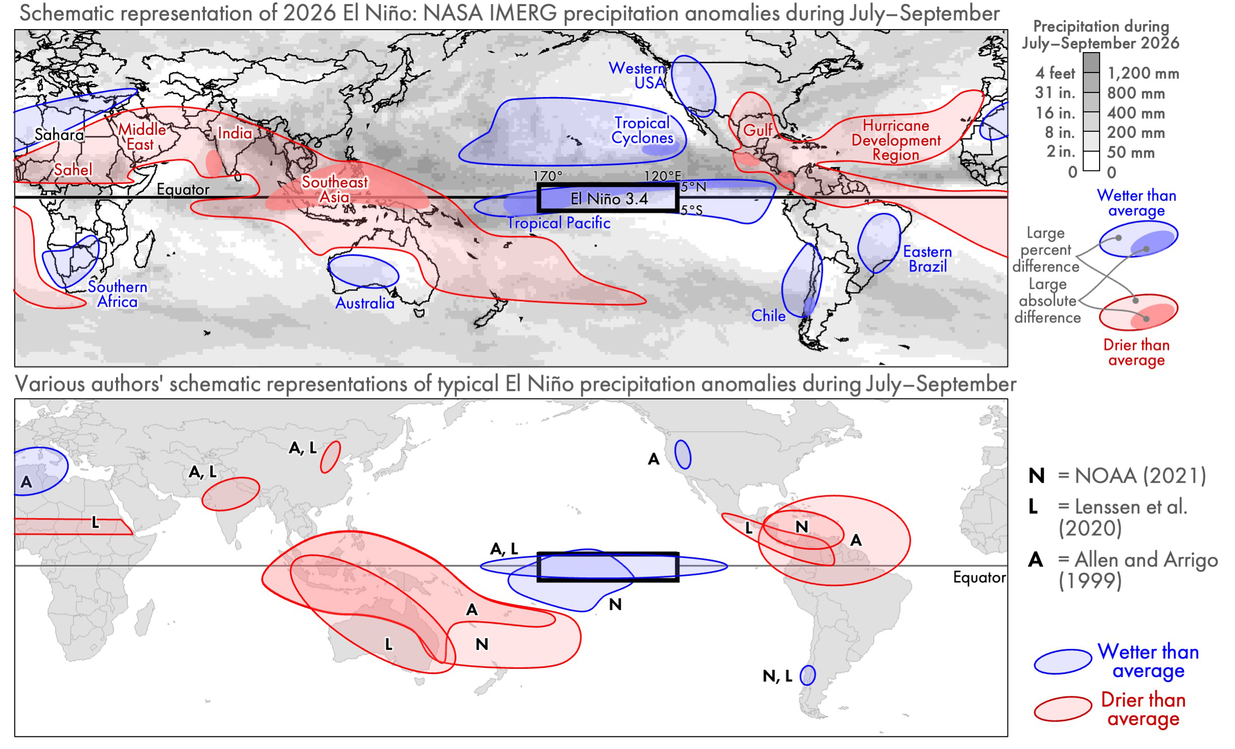
Figure 9. Schematic diagrams of El Niño’s effect on precipitation: anomalies during July–September 2026 described in this article (top) or anomalies associated with prior El Niños during July–September (bottom) [High-res image]

The top panel of Figure 9 is a schematic diagram that summarizes the anomalies seen in IMERG precipitation estimates. Light blue and red regions indicate percent anomalies, i.e., where there was much more or less precipitation than usual, expressed as a percent of a location’s long-term average for July–September. Dark blue and red indicate regions where the 2026 anomaly was large in absolute terms, i.e., in units of millimeters of accumulation. The gray background provides context by showing the total precipitation accumulation during these three months in 2026. Regions where anomalies are large in absolute terms (dark red or blue) are generally a subset of the locations where it rains a lot anyway (dark gray).

The bottom panel of Figure 9 shows what three other authors identified as typical El Niño impacts on precipitation during July to September. Different schematic diagrams may agree in some places while disagreeing elsewhere. Such differences are to be expected because a schematic is inherently a simplification and is intended to emphasize certain aspects of a phenomena.

The three authors agree that, during this time of year, El Niños are associated with drought in Southeast Asia and Central America. They agree that El Niños are associated with above-average rainfall in the portion of the tropical Pacific defined as the Niño 3.4 region. Yet, these authorities disagree about where else precipitation anomalies are to be expected during an El Niño. In the bottom panel, the labels N, L, and A, refer to the anomalies identified by NOAA (2016), Lenssen et al. (2020), and Allen and Arrigo (1999).

The Columbia Climate School has published a different style of schematic that summarizes, in a single diagram, El Niño’s precipitation impacts in every season, not just a single three-month period. Their diagram depicts the most widely known El Niño impacts, which might lead to confusion when reading the present article. The present article shows an unusually dry southern United States and wet southern Africa, yet the Columbia diagram suggests that the opposite is expected. The reason for the difference is that these features in the Columbia diagram are anticipated later in the year, not during the July–September period covered in the present article.

Instead of comparing different authors’ schematic diagrams, one could evaluate the reasonableness of the IMERG-estimated El Niño impacts by comparing them to the output of an atmospheric model. On June 21, climate researcher Erik Kolstad wrote about a forecast from the ERA-5 model, which is version 5 of the reanalysis model developed by the European Centre for Medium-Range Weather Forecasts (ECMWF). One of the ERA-5 forecast maps is show below, along with a reprojection of the IMERG data discussed in the present article.

Figure 10. The 2026–27 El Niño’s impact on precipitation as IMERG observed in July–September (top) or as ERA-5 forecasted would occur during June–August (bottom) [High-res image]

The bottom panel of Figure 10 shows results from the ERA-5 model. Covering June–August 2026, the figure shows where ERA-5 forecasted that precipitation anomalies would be positively correlated with Niño 3.4 sea surface temperature (SST) anomalies. Where precipitation and SST are positively correlated, one should expect above-average rain accumulation during an El Niño. Where these quantities are negatively correlated, one should expect below-average rain accumulation during an El Niño. The top panel of Figure 10 shows the previously discussed IMERG precipitation anomalies for July–September 2026. Excluding locations near the North or South Poles, the sign of the precipitation anomaly is the same in many places when IMERG and ERA-5 are compared.

Variation in Societal Impact

The magnitude of a precipitation anomaly does not, by itself, determine the magnitude of societal harm, such as to the economy or infrastructure. Other factors modify disaster risk, including population density and how susceptible local infrastructure is to extreme weather (Carrao et al., 2016). To summarize the preceding discussion, some precipitation anomalies during July–September 2026 are listed below along with a brief statement about their societal impacts.

IMERG estimated that parts of southern Africa and western Australia had more than double their normal precipitation during this period, but there were no reports that the extra precipitation caused any major catastrophes (ABC News, 3 Oct 2026). IMERG also estimated more than double normal rainfall over Chile during this part of 2026, and damaging floods were reported there (Reuters, 28 August 2026; Mining Reporter, 21 July 2026).

IMERG estimated a 20% deficit of rainfall over western India during July–September 2026. The media reported that India’s harvest was the worst in a decade, which caused hardship (Down to Earth, 30 Sep 2026; South China Morning Post, 1 Oct 2026). Based on a dense network of thousands of rain gauges, the Indian Meteorology Department provided independent confirmation of this part of the global pattern seen by IMERG. During June through September, the Department estimated that rainfall was about 10–30% lower than average over most of India’s subdivisions in the western third of the country (IMD 30 Sep 2026, Figure 3a).

Similarly, IMERG estimated a more than 20% deficit of rainfall over Southeast Asia during this part of 2026. The media reported a drought here that caused water shortages and threatened food security (PBS News Hour, 22 Sept 2026).

In 2026, much of the eastern Sahara Desert and Saudi Peninsula had less than half of their normal July–September accumulation, yet there were no reports of major economic harm from a drought. Confirming this part of the global pattern seen by IMERG, a near real-time rain-gauge dataset (Figure 3) reported rain deficits of ≥50% in similar areas in the Middle East and Southeast Asia. Extremely arid portions of the Middle East do not depend on current-year rainfall for drinking water, and rain-fed agriculture is an insignificant part of their economy.

The patterns described in this article are based on NASA’s precipitation estimates made in near real time, which means within about 15 hours of when the satellite observations were collected. These estimates were made independently of rain-gauge observations for the current month because it takes several months for a quality-checked global archive of monthly rain-gauge accumulation to become available in a form that the IMERG algorithm can use as an input. NASA generates these real-time satellite-based estimates using a simplified algorithm called the Late Run of IMERG. The analysis in this article should, therefore, be considered preliminary, subject to revision once the Final Run of IMERG becomes available in several months.

Final Thoughts

El Niño is one of the Earth’s many oscillations and cycles that affect precipitation and that occur naturally on time scales of a day to several years. NASA’s IMERG algorithm provides global, near real-time estimates of precipitation that are useful, among other things, for monitoring the El Niño that is expected to last from summer 2026 to spring 2027. The CEOSR team carried out this preliminary analysis of the current El Niño as observed by IMERG during July to September 2026.


El Niño and MJO: Oscillations in Global Precipitation

GMU’s CEOSR team assists NASA with testing new versions of satellite data-processing algorithms and monitoring the output of the operational version. Some of these same analysis and display tools can be used to explain to the general public the patterns that exist in the decades of NASA’s global rainfall estimates.

One pattern that emerges every two to seven years is an El Niño, a phenomenon that has been in the news during 2026 because a strong El Niño formed during the summer. This article shows how past El Niños have affected the global distribution of precipitation. It also compares El Niño to another natural oscillation called the Madden-Julien Oscillation (MJO). The MJO has similarly large impacts on global precipitation but is much more frequent, repeating every few weeks or months.

Background

Whether or not it rains a week from now where you are may seem mostly random, but a long enough data record will likely reveal rainfall patterns that repeat over hours, months, or years.

Atmospheric scientists describe some of these repeating patterns as cycles and others as oscillations. There are annual and daily precipitation cycles tied to the variation of the sun’s path across the sky.[1] An example of precipitation affected by time of day is that summer thunderstorms occur predominantly in afternoon or early evening along the East Coast of the United States. An example of seasonal precipitation is that the U.S. Southwest has mountains receiving most of their precipitation as winter snowpack and lower-elevation areas receiving most of their precipitation in late summer. A prior article on the GPM website describes how precipitation cycles are tied to the sun.

This article describes two precipitation oscillations that impact the economy.[2] In most cases, atmospheric scientists use the term “oscillation” rather than “cycle” to describe less regular but repeating patterns that are driven by hard-to-predict and complex processes in the atmosphere and ocean.[3]

A good dataset for studying precipitation oscillation is IMERG, which is created by NASA’s Global Precipitation Measurement (GPM) Mission. IMERG stands for Integrated Multi-satellitE Retrievals for the GPM Mission. Starting with January 1998, IMERG provides estimates of the rate of rainfall and snowfall every half hour and every 0.1 degrees of latitude and longitude. This resolution equates to individual measurements covering areas about 7 miles across or smaller.

The best known precipitation oscillation may be El Niño, which is a Spanish word, so “Niño” is pronounced “neen´ ee-oh.” For centuries, sailors have used the term El Niño to refer to events when the ocean off Ecuador’s coast is unseasonable warm in December. In the 1960s, scientists realized that El Niño events were part of a larger phenomenon that also includes the Southern Oscillation. The Southern Oscillation is characterized by a variation in wind and pressure in the Equatorial Pacific. It can alter the strength of India’s summer monsoon rain among other effects.[4] India closely monitors the monsoon because food insecurity may result if the monsoon fails one year or is marked by more flooding than usual. To describe the full El Niño / Southern Oscillation system, scientists use the acronym ENSO.

In some parts of the world, another oscillation is also well known, specifically the Madden-Julian Oscillation (MJO). In countries where rainfall is particularly affected by the MJO, such as Australia, weather reports mention it regularly. When a strong MJO event unfolds, it can intensify the impacts of ENSO in some places and mask them elsewhere.

Both ENSO and MJO will be discussed in more detail below. Incidentally, scientists pronounce ENSO as a word, as in “en´ sew,” while they pronounce MJO letter-by-letter, as in “M J O.”

Monitoring Atmospheric Oscillations

An atmospheric oscillation repeatedly passes through a set of well-defined phases, but the duration of an individual phase can vary and sometimes the phases occur out of their normal order. These recurring phases are each associated with a complex pattern of air pressure, wind, temperature, and precipitation. To make it easier to identify which phase exists at any given time, an index is calculated from observations using an agreed-upon formula. As scientists improve our understanding of the atmosphere, they propose new formulas to serve as oscillation indices.

The phases of an oscillation may be named or numbered, as shown below for the first years of the IMERG dataset. Click here for a plot that covers a longer period.

During 1998 to 2003, the phases of ENSO (top) and the Madden-Julian Oscillation (bottom). The cycle of the months of the year is shown in the middle.

The three phases of ENSO are named El Niño, La Niña, and neutral. Since the 1990s, a frequently cited index for ENSO is the deviation from average conditions of the ocean surface’s temperature in a region of the central Pacific. This region of the ocean is called Niño 3.4, and it covers 5°N–5°S latitude and 170°–120°W longitude. NOAA uses buoys and ship observations to precisely measure the ocean’s temperature. Because several oscillations operate on a similar time scale as ENSO, the index for ENSO is based on observations in the region that best isolates the ENSO signal.

Instead of having names, the eight phases of the Madden-Julien Oscillation are numbered 1 through 8. Over the past decade, an index called OMI has been widely adopted to calculate if one of the MJO phases is present or if the atmosphere is in an inactive state with respect to the MJO. OMI stands for the outgoing longwave radiation (OLR) MJO index. Using satellite observations, the OMI compares current observations of global cloud-top temperature against precalculated patterns. These precalculated patterns were generated from cloud-top observations spanning many years.[5] These patterns capture the strongest variation in cloud-top height globally, on the time scale of several weeks to months. A global index, rather than a regional one, works for identifying the phase of MJO because the MJO is the strongest oscillation at this time-scale anywhere on Earth.[6]

Oscillations that Repeat Every 2 to 7 Years

It usually takes ENSO 2 to 7 years to pass once through its two active phases, El Niño and La Niña.

ENSO’s impact on precipitation is best seen in anomaly maps. To calculate an anomaly, first calculate a map of the average precipitation during El Niño years and a separate average for La Niña years. From these two maps, subtract the long-term average annual accumulation at each location over a long period that includes El Niño, La Niña, and neutral years.

It is worth noting that using the term anomaly for the precipitation variation associated with El Niño does not imply that anything unexpected, alarming, or mysterious is occurring. In atmospheric science, an anomaly is merely a statement that current conditions deviate from average conditions. Anomalies occur all the time basically everywhere because rain in any given year is almost always at least a bit more or less than the long-term average.

One way to ensure that an anomaly map reveals the full geographic range of ENSO is by using units of percent deviation from each location’s average precipitation accumulation. Percent deviation highlights different features than does an anomaly map expressed in absolute terms, with absolute meaning millimeters of precipitation per year. It rains a lot each year near the Equator, and there are large variations in the absolute amount of rainfall there from one year to another. The absolute amount of rainfall is generally much less over the rest of the Earth, but the percent change in rainfall can be just as large from year to year. A large percent change can have a large impact on agriculture and ecology, so a percent-anomaly map is a useful tool both near and far from the Equator.

The following figure shows a percent-anomaly map for El Niño and another for La Niña. To generate this figure, only moderate and strong events during 1998–2025 were included in the calculation.[7] Dark red or blue indicate a large anomaly, which in this context means accumulation that is 50% below or above a location’s average annual accumulation.

The precipitation anomaly during El Niño or La Niña years seen in IMERG data during 1998–2025. [High-res image]

The IMERG image above shows that El Niño and La Niña both alter precipitation in locations far from the Equatorial Pacific. Scientific studies have documented impacts in California, Brazil, and Nicaragua (Chavda et al., 2023; Tien et al., 2025; Mendez-Rivas et al. 2024). The El Niño image above suggests that El Niño is associated with increased precipitation over East Africa, the Persian Gulf, and Central Asia. To the east, it is associated with decreased precipitation over India, central China, and Australia. Further east, it is associated with increased precipitation over the southeastern United States and Uruguay and decreased precipitation over Brazil.

In July 2026, NOAA forecasted an 82% chance of a very strong El Niño occurring in the autumn of 2026. If a very strong El Niño does start in 2026, it would be only the second time since the IMERG dataset began in 1998. The other time was in 2015–16.[8] The previous very strong El Niño reached maximum strength during the autumn of 1997, a few months before the IMERG dataset began.

The many years that separate strong El Niño events should be considered when designing a multi-satellite precipitation-estimation algorithm like IMERG. Such an algorithm should be designed to use input data that is available over a period that is long enough to contain an adequate sample of the full range of possible ENSO conditions.

Oscillations that Repeat Every 20 to 90 Days

The Madden-Julien Oscillation is a disturbance in which a large, loose cluster of storms interact with large-scale wind patterns and ocean circulation. The MJO’s strongest signal is generally near the Equator in the western Pacific. To put the MJO in context, it is sometimes described as a rapid oscillation superimposed on a slow oscillation; the slow oscillation being ENSO. Generally speaking, the MJO takes about 20 to 90 days to pass once through its eight phases. Scientific studies have used IMERG to study the MJO.[9]

The MJO was named after two scientists who drew attention to it in a 1971 paper. Today, the MJO is tracked by weather forecasters and atmospheric scientists because, among other things, it impacts tropical cyclones and other severe weather. For a few weeks every few months, the phase of the MJO may increase the likelihood of occurrence and severity of tropical cyclones in part of the world.[10] But when the MJO is inactive, no such impacts occur.

Dangerous impacts may occur when the enhanced precipitation associated with the MJO passes over a region that is already experiencing enhanced precipitation because of ENSO. When the two oscillations reinforce each other, the situation is somewhat analogous to how rough seas cause more coastal damage during high tide. In this analogy, individual waves are the rapid oscillation and the tide is the slow oscillation.

To generate the MJO animation shown below, several mathematical transformations are applied to IMERG precipitation estimates. These transformations isolate the 20-to-90-day signal from other precipitation oscillations that proceed more slowly or rapidly.[11]

An animation showing the precipitation anomaly during the eight phases of the 20–90-day oscillation during the Northern Hemisphere winter (top) and summer (bottom). Credit: Jason West.

The geographic pattern of precipitation anomalies that repeat every 20–90 days is influenced by the season (Kiladis et al. 2014). For this reason, many scientists now use a different term for the 20–90-day oscillation during the two halves of the year. This practice follows the recommendation of Shukla (2014) that the term MJO be reserved for November through April, while the term Monsoon Intraseasonal Oscillation (MISO) be used during the other half of the year.

Several indices have been proposed for determining which, if any, phase of the 20–90-day oscillation is active on a particular day. One popular index is called OMI and it is sensitive to tall, vigorous convective rain cells. Such storms are more common during summer than during winter. For this reason, the hemisphere experiencing its warm season tends to be the hemisphere with the largest 20–90-day anomalies. During phase 1 of the oscillation, the animation above shows that Northern Hemisphere summer (bottom panel) experiences increased precipitation over the East China Sea and south of Mexico, and decreased precipitation over India. During Southern Hemisphere summer (top panel), phase 1 exhibits an increase in precipitation northeast of Fiji and over Brazil, and a decrease just north of Australia.

Scientists use various techniques to visualize the MJO, one of which is longitude-time diagrams. The longitude-time diagram below shows that the precipitation enhancement (blue) moves to the right (toward the east) along the Equatorial Indian and Pacific Oceans as the MJO phase passes from 1 to 8.

A longitude-vs-time cross section of IMERG precipitation anomaly along the Equator associated with the phase of the MJO during 1998–2024

One method for checking the validity of satellite-observed precipitation is to compare it against observations made with weather radars on the ground. This technique works only over the small portion of the Earth within range of a ground radar. The MJO pattern seen in IMERG data is similar to the pattern seen in NOAA’s Stage IV ground-radar-based precipitation estimates over the United States. Consistent with both IMERG and ground radars, research shows that part of North and South America have enhanced precipitation during phases 8 and 1 and reduced precipitation in phases 6 and 7.[12]

Reaching into Arid Regions

The images and movies discussed so far for the 20–90-day oscillation show precipitation anomalies mostly in areas that receive a lot of rain each year. In fact, precipitation anomalies extend into arid regions as well, but a different visualization technique is needed to see them. The image below show regions that receive little rain during May through October, i.e., the warm half of the year for the Northern Hemisphere. These arid areas are similar but not the same as those during the other half of the year that includes Southern Hemisphere summer.

Map of arid regions during Northern Hemisphere summer based on IMERG data from 1998–2025. [High-res image]

The yellow regions in the above image are where no more than 9 inches of rain falls during May through October, on average. In comparison, this amount is less than half of the typical May-to-October accumulation over the United States East Coast.

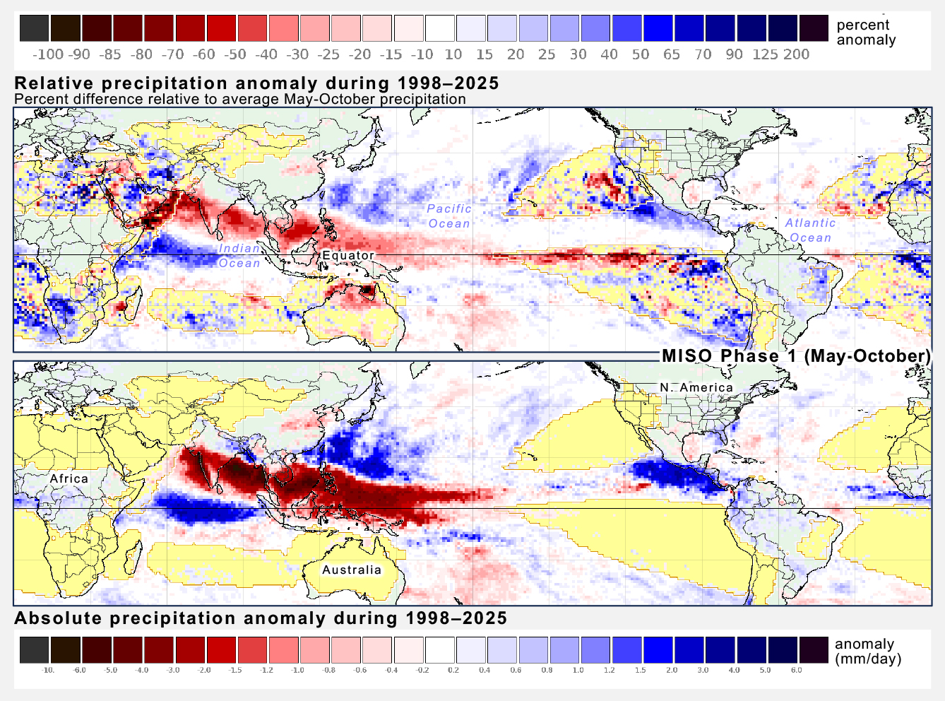
In the image below, the top panel uses percent anomalies to show how MISO’s influence on precipitation extends into arid regions. Deep red or blue shows where precipitation during phase 1 of MISO is 50% lower or higher than normal, respectively.

Comparison of relative and absolute anomalies during MISO Phase 1. [High-res image]

In deep red, the bottom panel shows a precipitation deficit over India using an absolute scale, but the top panel shows that this deficit actually extends all the way onto the Arabian Peninsula using a percent-anomaly scale. In deep blue, the bottom panel shows excess precipitation near the Equator next to South America and Africa, but the top panel shows that this excess actually extends onto some of the arid regions of these continents if percent anomalies are displayed.

Final Thoughts

The long record and global extent of NASA’s IMERG dataset make it useful for studying how precipitation is affected by the El Niño / Southern Oscillation and Madden-Julian Oscillation. For both oscillations, their strongest precipitation signal is an east-west displacement of precipitation in the tropics over the Indian and Pacific Oceans. Percent-anomaly maps show that these oscillations also affect precipitation in the Northern Hemisphere’s subtropics and midlatitudes where most of the world’s population lives (23.5–66.5ºN latitude).

There are several considerations that motivate scientific study and operational monitoring of atmospheric oscillations. For example, food production depends on the timing and amount of rain. Severe storms periodically threaten property and lives in many parts of the world.


Notes

[1] The annual and diurnal cycles of precipitation are very different things than the water cycle. The water cycle is a sequence of steps by which water flows from on or below the Earth’s surface to the atmosphere and back. Precipitation is one step of the water cycle.

[2] On June 17, 2026, Fortune Magazine published an article that mentioned a 2023 scientific study published in the journal Science that found that a powerful El Niño can cause $6 trillion of harm to the world economy. This article discusses El Niño and MJO. MJO is sometimes described as a high-frequency perturbation on top of El Niño, so just as El Niño has economic impact, so does MJO.

[3] The distinction made here between precipitation cycles and oscillations isn’t found in most textbooks or websites, but it is made informally when atmospheric scientists talk among themselves. That being said, a few scientific papers treat the terms oscillation and cycle if they were interchangeable. While discussing variation in precipitation, Grimm (2019) refers to the “cycle” of the Madden-Julian Oscillation. Liu et al. (2020) and Gutzler et al. (2002) mention the “El Niño-Southern Oscillation cycle”.

[4] Enfield (1989) discusses the history of when scientists realized El Niño events were connected with the Southern Oscillation.

[5] Kiladis et al. (2014) published the definition of the OMI, which stands for outgoing longwave-radiation (OLR) MJO index. The values of OMI can be found on the NOAA Physical Sciences Laboratory’s MJO page.

[6] Even though scientists use a single index for the MJO during all months of the year, some scientists calculate separate rainfall anomalies for northern-hemisphere and southern-hemisphere summer: November-April and May-October. They call one anomaly MJO and the other anomaly MISO. This distinction is made later in this article.

[7] The software that generated these images used Jan Null’s list of years with moderate or strong El Niño or La Niña events. The software averaged IMERG precipitation during the 12 months associated with each event, taking observations from July of the year that the event started through June of the next year. This 12-month period is chosen because ENSO events tend to reach their maximum strength within a few months before or after December.

[8] Santoso et al. (2017) discuss the 2015-2016 El Niño which was the strongest one since the 1997-1998 El Niño. An article on the GPM website describes IMERG observations of the 2015-16 El Niño.

[9] Bai and Schumacher 2022 and Xianan et al., 2020.

[10] The MJO’s ability to influence severe weather is mentioned in Klotzbach et al. (2023) and in an earlier post to the GPM website about Tropical Cyclone Ana (2021).

[11] First, the 28-years of 24-hour IMERG estimates has its linear trend removed. Then, the seasonal cycle is subtracted. This means calculating the average precipitation rate for a given day of the year and subtracting that average from the 28-years of data. The 20-to-90-day variations in precipitation are extracted from the time series using the Lanczos bandpass filter. An index is used to identify the days in the time series that have a strong expression of one of the eight MJO phases (an OMI amplitude of ³1). The average precipitation is calculated separately for each phase and for the Northern Hemisphere summer or winter. The MJO index used in this analysis is NOAA’s ROMI, which stands for Realtime Outgoing Longwave Radiation (OLR) MJO Index.

[12] For the North and South America pattern, see Figure 12 of Fernandes and Grimm (2023). A less technical account is provided by Arcodia (2020).


Monitoring in 3D: Typhoon Sinlaku (2026)

In April 2026, Typhoon Sinlaku impacted the Pacific Islands of Guam, Saipan, and Tinian. As the storm approached the islands and made landfall, NASA’s Global Precipitation Measurement mission (GPM) satellite and multi-satellite data-processing algorithms gave insights into the rain that fell from this powerful storm. Now, learn how GPM helps us go beyond individual snapshots of surface rainfall by observing Typhoon Sinlaku over time and through the depth of Earth’s atmosphere.

The Time Dimension

Because of technological limitations, satellite instruments that see into a storm don’t hover over one place on Earth. Instead, they capture a snapshot of a storm as the satellite rapidly orbits the planet at a speed of about 5 miles per second. To build up the life story of an individual storm, it is necessary to stitch together observations from many satellites. Since 2014, NASA has done so by running the IMERG multi-satellite precipitation-estimation algorithm, which NASA developed in collaboration with scientists at other agencies and universities.

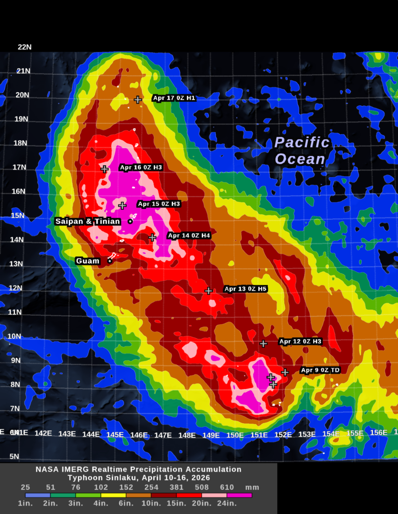
The movie below shows seven days of rainfall from Typhoon Sinlaku. This animation is built up from estimates made every 30 minutes from April 10 through April 16. In this movie, the transparent gray clouds represent Geosynchronous infrared satellite observations and the rainfall rate shown in color comes from NASA’s IMERG algorithm. These IMERG estimates can be viewed in NASA’s RAIN-Global 2 web tool or on the WorldView webpage.

These 30-minute surface rainfall rates can be summed to arrive at the storm-total rainfall accumulation. The public, businesses, and disaster agencies care about storm totals, not just when a storm will hit, so accumulation comes up in weather discussions. At about 2PM EDT (01800 UTC) on April 13, the National Weather Service office for the island of Guam warned the public that Typhoon Sinlaku could bring 15 to 25 inches of rain to the nearby Pacific islands of Saipan and Tinian in the subsequent days.  In its hurricane local statement, the Guam office said that passive-microwave satellite observations influenced their prediction.

The 7-day accumulation shown above is one way to illustrate how the National Weather Service may have arrived at its 15-to-25-inch forecast.  During the two days before Typhoon Sinlaku reached Saipan and Tinian, the IMERG algorithm estimated that the storm was dumping about 6 to 20 inches of rainfall along the portion of its track southeast of these islands. This range is shown in orange and red in the image. The typhoon’s forward speed was cut in half around the time it started impacting Saipan and Tinian, which would increase the time it would spend over these islands. Other factors remaining equal, a slower forward speed would proportionally increase the expected rainfall total. Where the storm center passed with a slow forward motion (during April 14–15), IMERG estimated that the accumulation was 20 to 30 inches (pink and magenta in the image).

In the 7-day accumulation image, the location of Sinlaku’s center is marked with a white plus sign at 0000 UTC, each day. The storm’s strength is indicated by H1 through H5 for categories 1–5 on the Saffir-Simpson scale or by TD, which stands for Tropical Depression.  

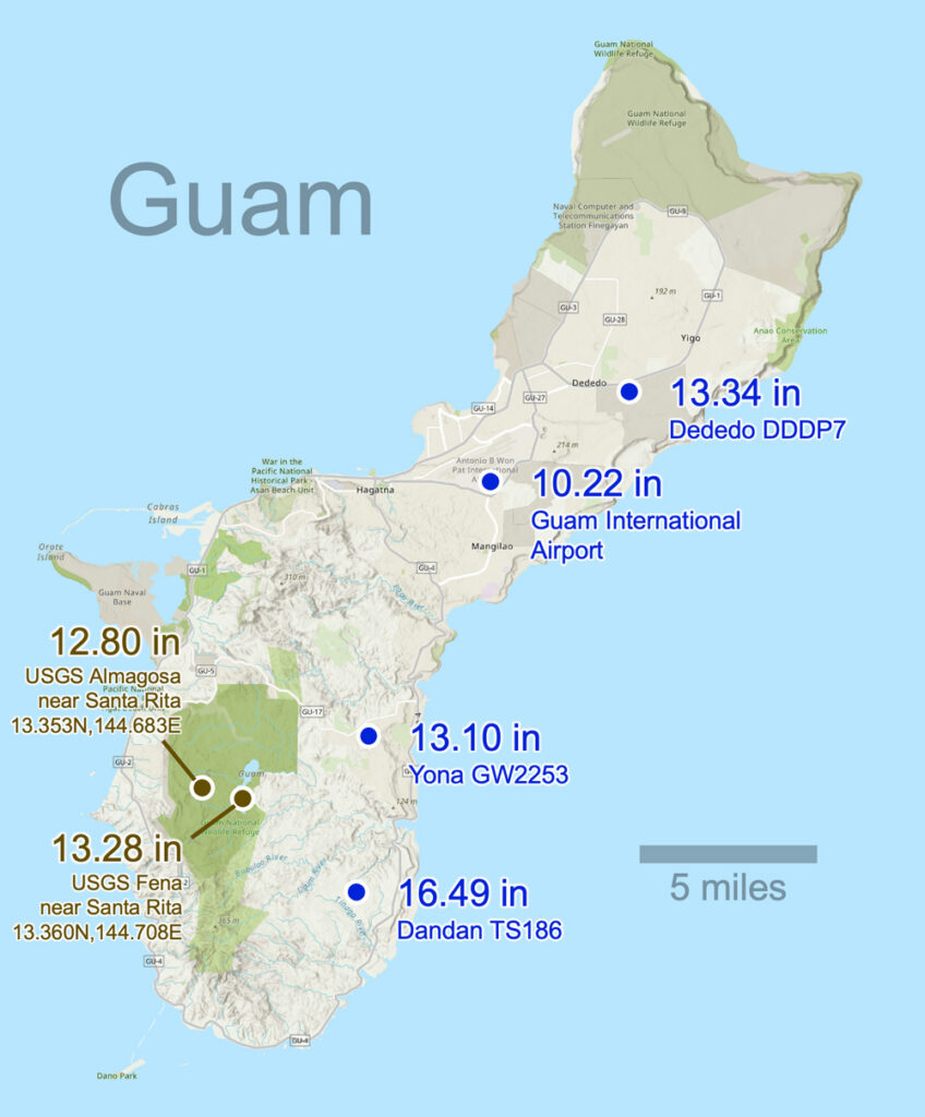
One way to increase confidence in these near real-time IMERG storm totals is to compare them to near real-time rain-gauge observations where available.  Rain-gauge data is not available immediately following Typhoon Sinlaku’s landfall for the two islands most severely impacted, Saipan and Tinian. However, just 130 miles to the south, several rain gauges in Guam continued to operate during the passage of Typhoon Sinlaku.  Between April 9 and 17, the National Weather Service and the USGS reported that six rain gauges in Guam had accumulations of 10.2 to 16.5 inches, respectively, including at Almagosa, Dededo, and Santa Rita. The map below shows the location of these gauges. IMERG reported 10 to 20 inches of accumulation over Guam, which indicates good agreement with these gauges. 

The Third Dimension

NASA’s Global Precipitation Measurement (GPM) Measurement satellite carries a radar built by Japan that is currently the only instrument in space able to observe the three-dimensional structure of storms. A few other cloud or precipitation radars are also in space, but they collect only two-dimensional curtains of data with data collected along the satellite’s direction of motion and vertically. The EarthCare and Tomorrow.IO satellites carry such 2D radars. Other satellite instruments collect different types of 2D data. Passive microwave instruments see into and through a storm, producing an image somewhat like a medical X-ray of the body. Infrared satellite instruments see only the top surface of a storm cloud, something like a hand-held infrared thermometer taking your temperature when pointed at your forehead. 

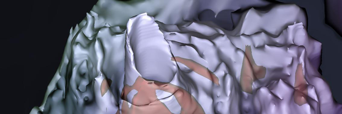
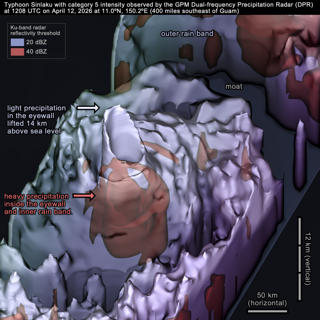
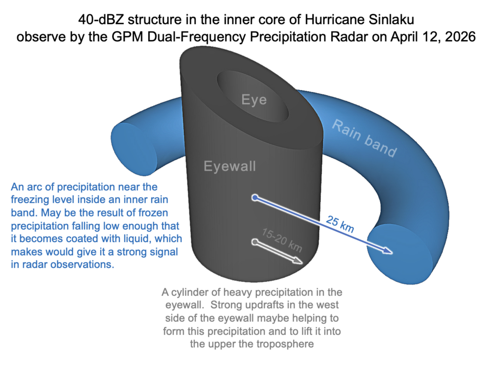
The dual-frequency radar on the GPM satellite flew over Typhoon Sinlaku’s eyewall on April 12, 2026. At 1208 UTC that day, the typhoon had reached category 5 on the Saffir-Simpson scale and would soon reach its peak wind intensity.

Above, the 3D image shows the radar-observed volume of the light precipitation inside Typhoon Sinlaku. Light precipitation is represented by the blue-gray surface. To a first approximation, the precipitation in the lower half of the hurricane (within 5 km of sea level) takes the form of raindrops. Above that, there are various forms of frozen precipitation because the atmosphere is so cold at those altitudes. The blue-gray surface is defined by a 20-dBZ radar-reflectivity threshold. Inside this surface, there is in inner volume of heavy precipitation that the image shows in red. The inner volume is defined by a stronger radar signal, i.e., a 40-dBZ threshold. Generally speaking, a radar signal this strong indicates heavy rainfall or large ice hydrometeors coated in liquid water as they fall through warm air.

One can gather clues about the updrafts and precipitation processes at work in the inner core of Typhoon Sinlaku by studying the shape of the radar echoes inside it. The following schematic diagram provides one interpretation of the 40-dBZ signal that the GPM DPR observed.

CEOSR at George Mason University assists the GPM science team with examining major precipitation events and evaluating and running precipitation-estimation algorithms. For more information about the GPM satellite and the IMERG algorithm, visit the GPM website: https://gpm.nasa.gov. Images and story by Owen Kelley (CEOSR). Animation by Jason West (NASA/PPS/KBR).


Natural Cycles in Global Precipitation: Daily and Yearly

In many places, the amount of that rain falls on a particular day or hour is influenced by multiple natural cycles that exist simultaneously on different time scales. One such cycle repeats every 24 hours, and another repeats every year.

The global extent of these cycles can be studied using NASA’s IMERG precipitation estimates that have been generated for 1998 to the present. Most of Earth’s precipitation falls as rain, and the rest falls as snow, hail, or other forms of precipitation.

The length of IMERG’s data record makes it possible to average out some of the random error and unrelated weather fluctuation.  For example, any 100-year storm that occurs around the globe each year would do more to obscure the underlying daily and annual cycle of rainfall in a dataset that was shorter than IMERG’s 28 years. IMERG stands for “Integrated Multi-satellitE Retrievals for the Global Precipitation Measurement (GPM) Mission.” The IMERG algorithm is developed by a team of scientists, most of whom are affiliated with NASA Goddard Space Flight Center (Huffman et al. 2023a, 2023b, 2023c).

IMERG precipitation estimates give a more complete picture of Earth’s natural cycles because the dataset has high resolution and global extent. IMERG covers both continents and oceans because it is input data comes from a constellation of satellites that observe the Earth in the microwave, visible, and infrared spectrum. Over decades, individual satellites have joined and dropped out of this constellation like the changing lineup of a professional sports team.

IMERG is available every 30 minutes, globally, at a resolution of no less than 7 miles. IMERG provides estimates every 0.1 degrees of latitude and longitude, which equates to about every 7 miles at the Equator and less near the poles.

As described in an earlier article, you can browse through all of these 30-minute snapshots by visiting NASA’s World View webpage. Natural cycles can be hard to see by flipping through a series of 30-minute estimates. These cycles are easier to see if one first calculates average conditions and then calculates the time-varying deviation from these averages.  This approach is followed here.

The Daily Cycle

During some seasons and in some places, the average amount of precipitation varies with the time of day. Atmospheric scientists call this type of variation the diurnal cycle, and IMERG has been used to study this cycle (e.g., Tan et al. 2019, Watters and Battaglia 2019, Xiong et al. 2025, and Patel 2020). The diurnal cycle during July is shown in the animation below for 70º South to 70º North latitude. A single month of the year was chosen for this animation because, in many places, the diurnal cycle is different in summer and winter.

Precipitation varies with time of day during July, averaging over 1998–2025. Click here to play the animation.

To reduce noise, each frame of the animation covers a 12-hour period. For example, the first frame is centered on 6 AM local time and summarizes IMERG observations for midnight through noon during all Julys between 1998 and 2025. Each 12-hour frame starts 30 minutes later than the prior frame, so the second frame covers 12:30AM at night through 12:30PM in the early afternoon.

For a particular 12-hour period, the image is white where the precipitation rate equals the average rate for the whole day. Deep blue or red indicates large deviations from average conditions. Specifically, deep blue indicates that the 12-hour period has a precipitation rate that is about 50% higher than average and deep red indicates a rate 50% lower than average. The color bar was constructed with units of percent deviation from average conditions. Doing so makes the diurnal cycle easy to see in deserts and other arid locations, not just places that receive more rain.

As you examine the daily-cycle animation, it is important to understand how time is represented. A single frame of the animation shows data for the same range of local times everywhere on Earth. In contrast, a snapshot of the Earth would always show the full 24-hour range of local time as a function of longitude.

The speckle of fine-scale variation that is seen in each of these 12-hour averages demonstrates the high variability of rainfall and snowfall in both space and time. More than a hundred thousand 30-minute IMERG estimates were averaged together to produce each 12-hour image, and even this approach is insufficient to smooth out fine-scale geographic variation due to the influence of individual storms. In the face of nature’s variability, only a broad picture of the global, daily cycle of rainfall emerges from IMERG, a data product that represents NASA’s effort to optimally combine 28 years of observations from a constellation of geosynchronous and polar-orbiting satellites.

The Daily Cycle over Land or Ocean

Below, a single frame is extracted from the previous animation in order to illustrate the rule of thumb that rain tends to fall over land in the late afternoon and over ocean in the early morning.

The physical basis for this rule of thumb is that, unless it’s cloudy, the sun warms the land surface throughout the day, creating maximum atmospheric instability in the afternoon. This instability can trigger storms that persist for several hours as they are carried by the prevailing winds. In contrast, the temperature of the ocean surface changes very little most days because it takes much more energy to increase the temperature of water vs. that of air. Over the ocean, the nighttime cooling of tops of clouds increases atmospheric instability and can trigger rainfall around sunrise. The image below shows these patterns in IMERG data.

Over Asia and North America, the percent difference calculated from the afternoon-evening precipitation rate (noon to midnight local time) minus the daily-average precipitation rate.

The image shows afternoon and evening rainfall, averaging observation made from local noon to midnight during all Julys from 1998 to 2025. In this image, many land areas are dark blue, which indicates it rains there predominantly in the afternoon and evening. In contrast, much of the ocean is dark red, indicating that little precipitation falls there in the afternoon or evening.

Mountains Affect the Daily Cycle of Precipitation

As just described, enhanced rainfall in the afternoon or evening is common over land, but mountain ranges can modify this pattern. For example, the Rocky Mountains have an early afternoon precipitation maximum, but strong storm systems triggered by these mountains often persist for hours as the prevailing wind carries them hundreds of miles to the east. The many storms that follow this track result in peak precipitation occurring later in the day east of the Rockies.

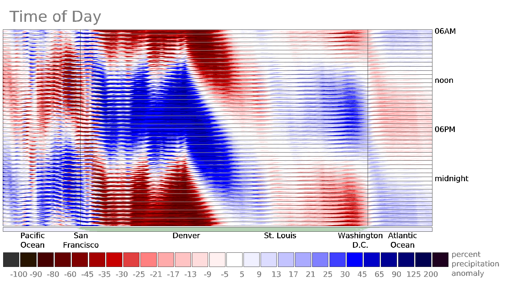
The Rocky Mountains’ impact is easy to see in the following cross section with longitude on its horizontal axis and time on the vertical axis. This kind of diagram is a called a Hovmoller diagram, and the one below is constructed for a west-east slice of the United States. The slice covers 35º to 40º North latitude, which includes San Francisco east to Denver, St. Louis, and Washington DC. The diagram combines all IMERG data for July during 1998–2025.

Looking at the diagram, it is clear that the rainiest part of the day is early afternoon in Denver and 12 hours later 850 miles east in St. Louis.

Precipitation variation over the United States in July during 1998–2025, as function of longitude and time of day.

The just described geographic variation of the daily cycle has implications for the constellation of satellites necessary to create global precipitation datasets that capture this natural cycle. It would not be possible to study precipitation’s diurnal variation with satellites that only observed the Earth at a fixed set of one or two local times in the afternoon and evening. During the IMERG era, Earth-observing satellites with microwave instruments, fortunately, have been stationed in a wide range of orbits, as depicted in an overflight-time plot generated by NASA.

One way to check that the diurnal patterns that IMERG sees around the globe are reasonable is by comparing them against regional high-quality independent datasets. For example, over the lower 48 states of the United States, there is a network of 150 weather radars operated by the National Weather Service. Data from these radars are shown every day on TV and online weather forecasts. Figure 6 of Sungmin and Kirstetter (2018) shows that this ground-radar data has a similar diurnal pattern to that shown in the IMERG diagram above.

The Annual cycle

Rainy and dry seasons exist are annual occurrences in some parts of the world. The timing of the wet season onset is economically significant and difficult to forecast. Scientists have used IMERG to forecast the onset and spatial pattern of the summer rainy season over India, West Africa, and Florida (Jayasankar and Misra 2025a; 2025b; Misra and Jayasankar 2024; GPM website). Other studies have used IMERG as a reference dataset to evaluate the accuracy of model forecasts of the rainy season over the watershed that supplies the Nile River (Gebremichael et al., 2025). Satellite-based precipitation estimates are the only hope here because there are too few rain gauges and weather radars in Africa for them to verify model forecasts of Nile River flow.

The following IMERG animation shows the annual cycle of precipitation across the world and has frames that each summarize a 30-day period. The first frame, for example, includes data from the first 30 days of 28 years (1998–2025). The next frame starts and ends two days later than the first frame. The yellow dot that moves north and south between 23.5°S and 23.5°N latitude indicates the latitude at which the noon sun is directly overhead during that time of the year.

As the previous section described for daily cycle, the animation below uses a similar red-blue color table to identify dry and wet anomalies in the annual cycle. For a particular 30-day period, the image is red or blue where the precipitation rate is less than or more than the annual average precipitation rate. In this way, this animation shows deviation from average conditions. In contrast, the GPM website’s Precipitation Climatology page shows the annual cycle of precipitation amount rather than the time-varying deviation from average conditions.

The annual cycle, showing how precipitation varies by day of year. To view the animation, click here.

As noted previously about the daily cycle, IMERG’s depiction of the annual cycle also contains strong small-scale variations that show up as speckles in the animation. NASA has expended considerable effort to extend the IMERG dataset back to 1998 in part because a long dataset is necessary to damp down the impact of individual weather events and to reveal underlying regional variation in the annual precipitation cycle.

The annual cycle and the sun

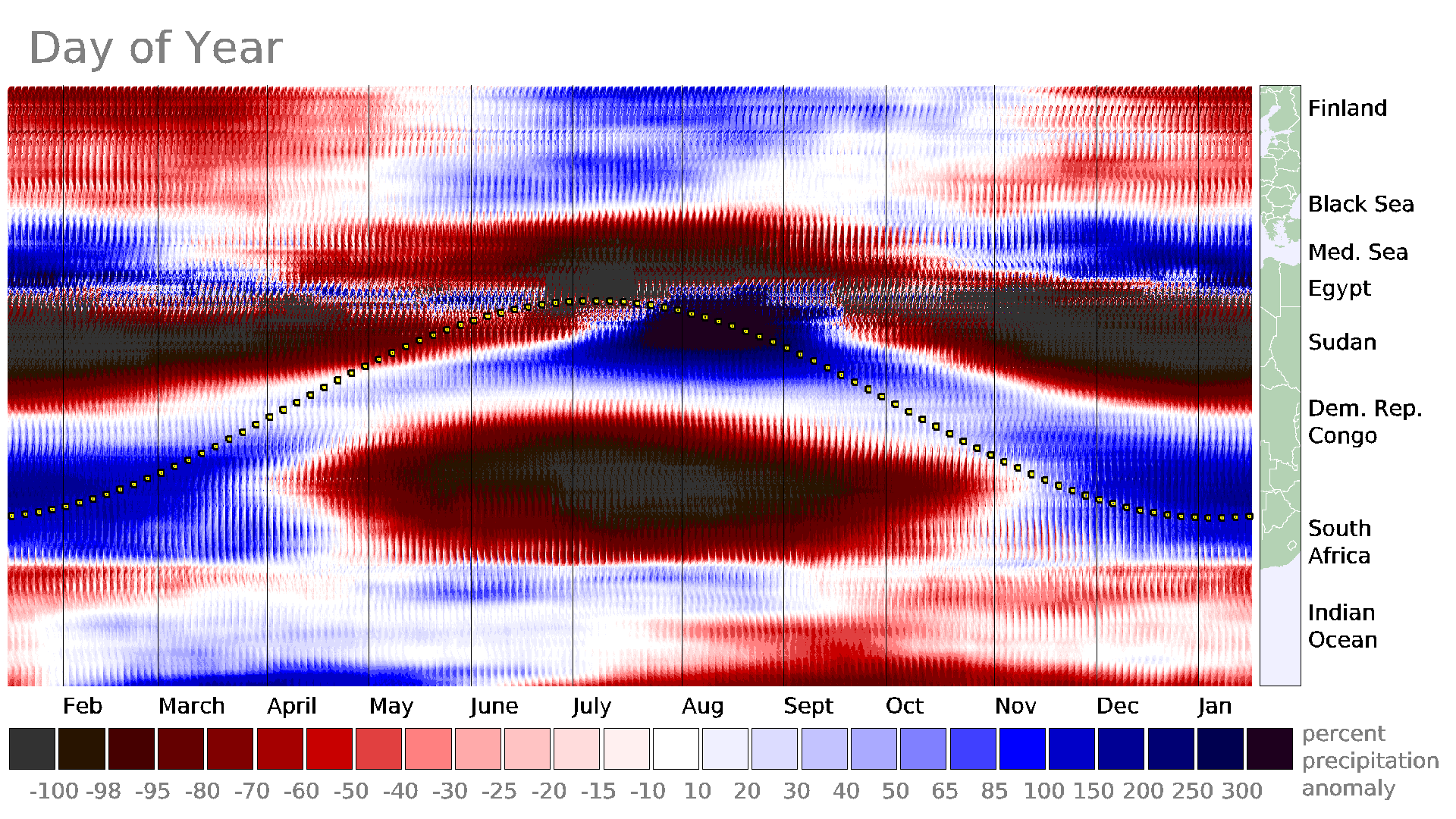
Over continents, there are many places that receive much of their rain during the summer. In both the Northern and Southern Hemispheres, summer starts in the part of the year when the sun is highest in the sky. This north-south migration of large precipitation accumulations can be seen in a time-vs.-latitude diagram, such as the one below. This diagram includes IMERG data from 50º to 60º East longitude, which includes locations from South Africa north to Finland. The line of yellow dots in this diagram shows the latitude at which the sun is directly overhead at noon.

A time-vs.-latitude cross section of the annual cycle of IMERG precipitation through a north-south section through Africa and Europe.

The rule of thumb that summer is the rainy season does not apply to ocean (Fig. 7, Huffman et al. 2023) or even to some land areas. For example, the image below averages data over the United States for all Januarys from 1998 to 2025. Blue over California, Oregon, and Washington indicates that January is typically a wet month on the West Coast. Red over the central United States indicates that little of the year’s precipitation falls there in January most years. The gray over the eastern United States indicates that precipitation in January typically accumulates at close to the average annual rate there.

Average January precipitation over the United States relative to annual-average precipitation.

Another way to explore the seasonal variation of precipitation over the United States is with a time-series diagram. Below is a time-series plot of three regions: the Pacific Northwest, the Great Plains of the central U.S., and the mid-Atlantic. The inset map shows these three regions. The horizontal axis is the day of year and the vertical axis is the long-term average precipitation rate for 30-day periods within the annual cycle. Each region’s median value is shown with dark dots, and the shaded area shows the middle 50% of IMERG values in the region. Cyan is used for Pacific Northwest, tan for the Great Plains, and light green for the mid-Atlantic region.

A time series for three regions of the United States that shows how their seasonal precipitation patterns differ.

Two of these three regions have peak precipitation near the time of the year that the sun is highest in the sky. The summertime peak is more pronounced over the Great Plains than over the mid-Atlantic. The Pacific Northwest, in contrast, has most of its annual precipitation fall in winter when it receives the least solar heating but is soaked by numerous storms coming off the ocean. A similar pattern is seen if the time series is calculated from NOAA ground-radar data (not shown) instead of IMERG data.

Final thoughts

NASA’s IMERG precipitation data contains daily and annual cycles. These natural cycles are easier to see if one examines deviations from average conditions. The daily and annual cycles are present in the 3.2 trillion precipitation values that make up the IMERG dataset for 1998 through the present.[1]

The IMERG algorithm is run and archived at NASA Goddard Space Flight Center. The Center also hosts the team of scientists who develops the IMERG algorithm. GMU’s CEOSR assists NASA both with evaluating the performance of the operational IMERG version and new versions before they become operational.


Notes

[1] 3.18´1012 IMERG precipitation values, which is derived from the following expression: (3600 longitude grid boxes) (1800 latitude grid boxes) (48 estimates per day) (365.25 days per year) (28 years).


Atmospheric River Strikes the Pacific Northwest

During the first three weeks of December 2025,several atmosphere rivers have carried plumes of moisture from the Tropics toward the United States. These plumes of water vapor have contributed to flood-producing storms over Washington State. The illustration below shows the approximate path that the moisture took to reach the United States.

Schematic diagram of an atmospheric river. [High-res image]

NASA’s IMERG algorithm stitches together observations from multiple satellites to estimate the precipitation that falls across the globe. IMERG stands for Integrated Multi-satellitE Retrievals for the Global Precipitation Measurement (GPM) mission. NASA’s Goddard Space Flight Center is home to the team of scientists who work to improve this algorithm and for the computing power that enables the algorithm to process more than a petabyte of observations.

To get a more precise idea of how much precipitation fell, the image below shows contours of precipitation accumulation during December 1 through 15. In this image, accumulation is measured in inches and is the sum of the depth of rainfall plus the depth of liquid that would be produced by melting any snowfall. This quantity is called the liquid-equivalent depth of the snowfall.

Precipitation accumulation over Pacific Ocean and the northwestern United States. [High-res image]

The above image shows two parallel trails of rainfall that stretch southwest to northeast across the Pacific Ocean. The northern trail reached Canada and the southern trail reached Washington State. These precipitation trails are evidence of the large amount of water vapor being transported along these routes, compared with the dryer air over nearby ocean regions.

Over the Pacific Ocean, the rainfall produced by these atmospheric rivers was fairly modest at 1 to 6 inches of accumulation during the first half of December 2025. The accumulation was more substantial over land. The large accumulations over North America were due in part to mountain ranges lifting the moist, oceanic, tropical air. IMERG estimated that the two-week precipitation total exceeded 15 inches over Washington’s Olympic Mountains, and further inland, the total exceeded 24 inches over parts of Washington’s Cascade Mountains.

During the first half of December western Washington suffered landslides, flooding, and power outages as a result of these atmospheric rivers. These storms also closed several highways that cross the Cascade Mountains. To see more clearly the geographic variation of rainfall, the zoomed-in image below shows just Washington State.

Close-up of precipitation over Washington State. [High-res image]

In the yellow-dotted region of the Cascade Mountains, a NOAA dataset broadly agreed with the NASA IMERG precipitation estimate, which is notable for two reasons. For one thing, much of the precipitation in this area fell as snow, which is more difficult to estimate from satellite observations than moderate rainfall. Second, any type of precipitation is difficult to estimate over mountainous regions, whether using ground radars, satellites, or rain gauges. NOAA generated its near real-time estimate over the United States using ground radars, rain gauges, and satellites. NOAA’s product is called “Stage IV.” IMERG’s near real-time estimates were generated over the whole globe using satellite observations calibrated against long-term gauge averages. The IMERG precipitation estimates also factored in the storm motion that was estimated from winds in a weather model.

Near the coast, the NASA and NOAA datasets diverged somewhat. Only the NOAA dataset saw a region of 24-inch accumulation over the Cascade Mountains, a compact mountain range west of Seattle. A rain gauge in the Cascades also reported over 24 inches of precipitation during the first half of December 2025, as indicated in the image by the cyan-color square. The two bow-tie-shaped symbols near Seattle indicate locations where the U.S. Geological Survey measured record river height. The rising water at these river gauges was a result of runoff from the heavy rainfall. The record river height occurred on December 11 and 12.


Large rainfall accumulation from Hurricane Melissa (2025)

Published October 29, 2025
Updated October 31, 2025

Hurricane Melissa Impacts Jamaica

An international constellations of satellites observed Hurricane Melissa as it passed over Jamaica on Tuesday, October 28, 2025.

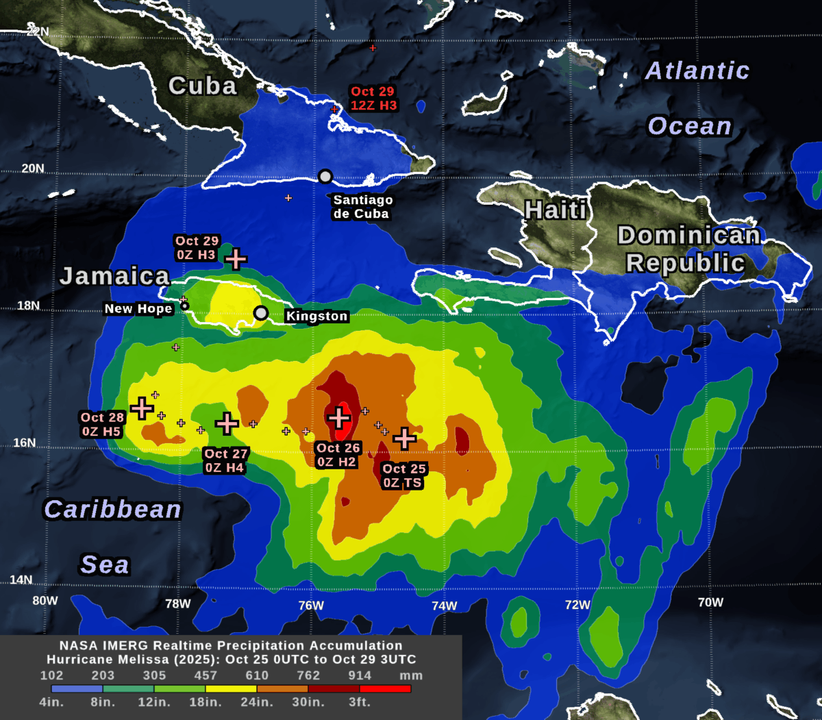
NASA’s IMERG algorithm combined rainfall estimates from these satellites in an effort to create the best possible estimate of rainfall in near real-time. IMERG stands for Integrated Multi-satellitE Retrievals for Global Precipitation Measurement (GPM). The image shows the depth of rain that IMERG estimated over land and sea during a little more than four days: 8PM EST October 24 to 11PM EST October 28 (in universal time, 0000 UTC on the 25th to 0300UTC on the 29th).

A day before landfall, the National Hurricane Center (NHC) forecast that the hurricane would dump 20-30 inches of rain on parts of Jamaica. This large amount of accumulation was expected because the storm was strong (category 5 on the Saffir-Simpson scale), the hurricane’s center was slow moving, and Jamaica has a mountain range oriented perpendicular to the flow of moist, oceanic air that the hurricane would force over the island.

The NHC rainfall forecast turned out to be broadly consistent with the near real-time IMERG estimates that were based on satellite observations.

By examining this storm and other severe weather events, researchers at George Mason’s Center for Earth Observing and Spatial Research (CEOSR) assist the team of scientists who develop the IMERG algorithm. This work is funded by NASA’s Goddard Space Flight Center. It includes helping to test new versions of the algorithm and searching for anomalies in the current version.

IMERG estimated that central Jamaica received 18-24 inches of rainfall during October 26-28, most of which occurred during October 28. This region is the yellow area over central Jamaica in the accumulation image at the top of this post, which can also be downloaded here.

During the preceding 48 hours, the center of Hurricane Melissa had stayed about 100 km south of Jamaica while it strengthened from category 2 to 5 and traveled slowly west. The plus signs in the accumulation image indicate the NHC’s estimate of the location of Hurricane Melissa’s eye every six hours.

The largest rain accumulations during this approximately 3-day-long period were over the ocean southeast of Jamaica, where IMERG estimated over 3 feet of rainfall. In the image at the top of this post, this region is show in bright red. The large accumulation there was caused by a combination of factors, including that rainfall was plentiful as the storm intensified over that location during October 26. Additional rain fell at this location after the hurricane eye had moved west because of a persistent precipitation feature that tracked to the east of the hurricane’s eye.

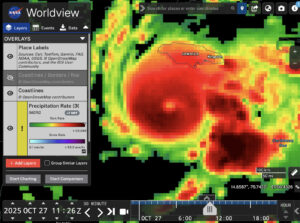
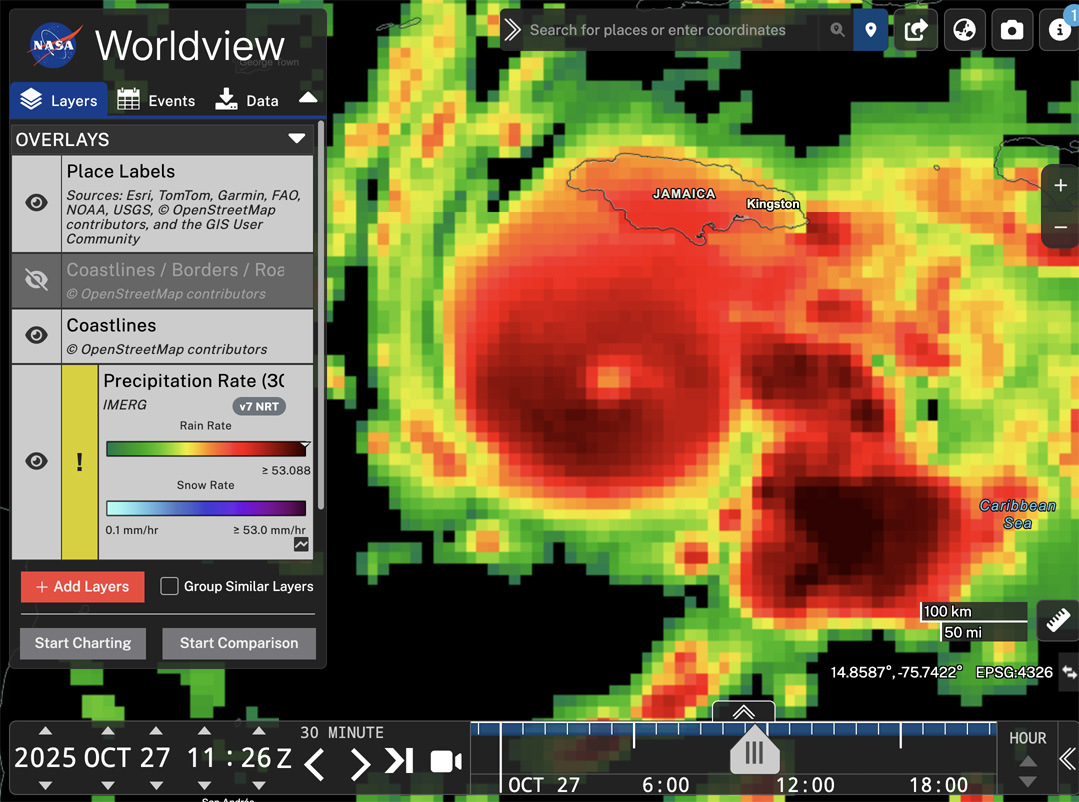
Hurricane Melissa (2025) in NASA WorldView (Oct. 27 1100UTC)

Snapshot of the IMERG rainfall rate estimate for Hurricane Melissa during 7:00-7:30 AM EDT on October 27, 2025 (1100-1130 UTC) . 

In the image above, this persistent stormy area east of Melissa is indicated with the arrow in the 30-minute precipitation-rate image. This image was captured from NASA’s Worldview web page. This image shows data from 16 hours before Melissa made landfall in Jamaica at approximately 1PM EDT (1700 UTC on October 28) according to the National Hurricane Center.  You can view a higher resolution version of this image here or interactively explore this data by following this link to Worldview.

Melissa Before and After Impacting Jamaica

The evolution of Melissa’s rainfall pattern can be tracked with the estimates available every 30 minutes from the IMERG algorithm. These estimates cover the globe with a resolution of approximately 7 miles (i.e., each grid box covers 0.1 degrees of latitude and longitude).

For October 23 through 29, the animation below shows heavy rainfall in dark red and cloud cover in shades of gray.

Animation of rainfall from Hurricane Melissa during October 23-29, 2025, as estimated by the IMERG algorithm. 

On October 23, Melissa was a tropical storm southeast of Jamaica with sustained heavy rainfall in excess of 25 mm/hr.  Smaller areas of heavy rainfall persisted after Melissa passed over Jamaica on October 28. They were mostly absent after Melissa traveled north of Cuba the next day.

At the end of the movie, the rain rates are hidden and the total 7-day rainfall accumulation is show in a green-purple color table. Despite the relatively lower rain rates over Cuba, total accumulations over eastern Cuba were still estimated to exceed 11.8 inches (300 mm) in some locations by the end of the day on October 29. These areas are shown in light purple. Accumulations in excess of 19.7 inches (500 mm) are shown in dark purple, and include large areas of the Caribbean Sea as well as central Jamaica.

When no satellite observations are available for a particular location and half-hour period, IMERG morphs satellite-observed precipitation from earlier or later times along the direction of the prevailing winds.

IMERG is ideal for monitoring hurricanes and other weather events that travel over land and ocean. Rainfall forecasts are available over the whole globe, but there are no rain gauges or weather radars nearby over the great majority of the ocean, so it is difficult to estimate how much rain actually falls there. Even over land areas with rain gauges, these measurements may not be available immediately after a storm strikes when disaster response must be organized.

For More Information

For more information about the IMERG algorithm, visit the website of NASA’s Global Precipitation Measurement (GPM) Mission. The Precipitation Processing System (PPS) at NASA Goddard runs the IMERG algorithm and distributes the data products.

Credits: Animation created by Jason West (KBR). Images created by Owen Kelley (GMU). Caption by Owen Kelley and Jason West.


Global Rainfall at Your Fingertips

CEOSR personnel working at NASA’s Precipitation Processing System (PPS) have generated 27 years of global rainfall imagery that is now available in NASA Worldview, which is NASA’s online archive of Earth science imagery.

NASA’s Worldview website now allows you to explore global estimates of rainfall and snowfall from 1998 to the present at 30-minute intervals. Researchers and application developers have been using this dataset since 2014 (Portier 2024; Portier et al. 2023), but now it is also available as images in Worldview.

This precipitation dataset is called IMERG, which stands for Integrated Multi-satellitE Retrievals for Global precipitation measurement (GPM). Over the years, a team of NASA scientists have improved the IMERG algorithm’s accuracy over land and ocean (Huffman et al. 2023a,b,c).

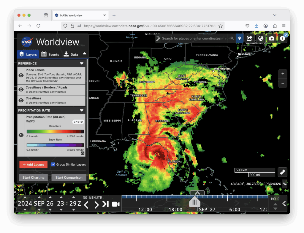
Worldview is now being updated every hour with the most recent global IMERG estimates. Worldview is a user-friendly website for visualizing many of NASA’s Earth science datasets. The image below shows the precipitation falling from Hurricane Helene shortly before it made landfall in Florida in September 2024 (West et al. 2024). In the image, you can see how the IMERG estimates cover land and also ocean where there are no rain gauges or ground radars.

Hurricane Helene, 30-minute precipitation, 26 Sept 2024 at 23 UTC
An IMERG snapshot of the precipitation falling from Hurricane Helene as displayed in NASA’s Worldview website. The estimate covers a 30-minute period near the end of September 26, 2024.

NASA runs the IMERG algorithm three times for each 30-minute period. The precipitation estimates from the first run become available just 5 hours after satellite observations are made, and that run is called Early IMERG. This near real-time dataset is useful for forecasting floods and monitoring large storm systems. A second run, called Late IMERG, occurs about 15 hours after observations are made. About four months later, the IMERG algorithm is run one last time when more observations and calibration datasets are available as inputs. This last run is called Final IMERG. Final IMERG is useful for studying droughts and other seasonal deviations from normal conditions. It can also be used for post-season reexamination of major events such as hurricanes. The Worldview website displays Final IMERG when available and Early IMERG otherwise.

Worldview for Beginners

If you haven’t used NASA’s Worldview website before, it is easy to learn how. Start by visiting https://worldview.earthdata.nasa.gov. There is no App to download, no user registration, and no charge.

When you visit Worldview, it initially loads satellite imagery of the most recent observations of the Earth’s surface and clouds. Precipitation is not initially displayed.

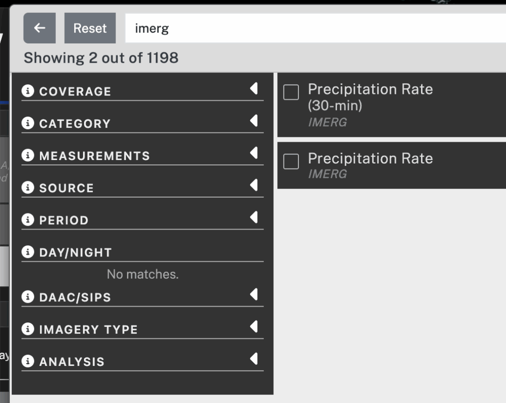
It takes two steps to display IMERG precipitation in Worldview. The first step is to add to your session the Worldview layer that contains 30-minute IMERG precipitation estimates. To do so, click the Add Layer button in the lower left corner. In the panel that pops up, type “imerg” in the search field. In the search results, check the box next to the entry for 30-minute IMERG. To dismiss the Add Layer panel, click the “X” symbol in the upper right.

Worldview Add Layer panel
The Add Layer panel in Worldview.

The second step is to move a few hours into the past.  To do so, you can move the time slider a little to the left in the timeline along the bottom of the Worldview window. Alternatively, you can use the arrow icons to move the clock display back a few hours. This time adjustment is necessary because IMERG precipitation estimates are created approximately 5 hours after satellite observations are made and it takes another hour or so to convert the data into Worldview imagery.

Worldview time bar
The date-time selection interface along the bottom of the Worldview window.

The 30-minute IMERG imagery should now be visible with green-yellow-red colors for rainfall estimates and cyan-blue-purple colors for snowfall estimates. To adjust the map’s zoom level, use the plus and minus buttons in the Worldview window or the scroll wheel on your mouse if you have one. To change the map’s location, drag the map with your mouse. By default, Worldview shows coastlines. For more detailed political boundaries and place labels, turn on optional layers. These optional layers can be found at the top of the layer list on the left side of Worldview.

The IMERG algorithm estimates the precipitation rate at the middle of each 30-minute period, i.e., 15 minute and 45 minute after the hour. The units of precipitation rate are the millimeters of rain-equivalent depth that would accumulate in an hour if the observed precipitation rate (rainfall or snowfall) were to persist for a full hour. If the precipitation is frozen, then the value that IMERG reports is the depth of liquid water that would result if the frozen precipitation were melted before its depth is measured. The liquid-equivalent depth of snowfall is relevant to the water storage in snowpack, which influences how much water will become available to plants once the snow melts. Because fresh snow contains air (i.e., it’s fluffy), about 4 to 20 inches of snowfall will melt down to just an inch of liquid water (Baxter et al. 2005).  IMERG states the liquid-equivalent depth of snowfall, but most weather reports state the depth of snowfall in its original, frozen form. 

One advantage to viewing IMERG precipitation imagery within Worldview is that one can hover over an image in Worldview to obtain a numerical range for the precipitation rate represented by that pixel of the image. The numerical range is displayed in the color bar on the left side of the browser window. This color-table-interrogation feature is available only if you are using a device with a mouse that can hover, such as a laptop or desktop but not a mobile device.

Worldview rain color bar
The Worldview color bar for rainfall. The downward-pointing white triangle indicates the color of the pixel in the IMERG image that is currently under the mouse pointer. The numerical range below the arrow is the range of precipitation rates associated with that color.

If you encounter any trouble downloading IMERG data, contact the GPM project using the contact page.

Credits: Story and visualization by Owen Kelley.

References

Baxter et al., 2005: A Climatology of Snow-to-Liquid Ratio for the Contiguous United States. Weather and Forestcasting, 20, 729–744, Figs. 3 and 5.

Huffman, G. J., D. T. Bolvin, D. Braithwaite, K. Hsu, R. Joyce, C. Kidd, E. J. Nelkin, S. Sorooshian, J. Tan, and P. Xie, 2023a: NASA Global Precipitation Measurement (GPM) Integrated Multi-satellitE Retrievals for GPM (IMERG) Version 07, Algorithm Theoretical Basis Document (ATBD). https://arthurhou.pps.eosdis.nasa.gov/Documents/IMERG_V07_ATBD_final.pdf.

Huffman, G. J., D. T. Bolvin, R. Joyce, O. A. Kelley, E. J. Nelkin, J. Tan, D. C. Watters, and B. J. West, 2023b: Integrated Multi-satellitE Retrievals for GPM (IMERG) Technical Documentation. white paper, https://arthurhou.pps.eosdis.nasa.gov/Documents/IMERG_TechnicalDocumentation_final.pdf.

Huffman, G. J., D. T. Bolvin, R. Joyce, O. A. Kelley, E. J. Nelkin, J. Tan, D. C. Watters, and B. J. West, 2023c: IMERG V07 Release Notes. white paper, https://arthurhou.pps.eosdis.nasa.gov/Documents/IMERG_V07_ReleaseNotes_final.pdf.

Portier, A., 2024: Using GPM Precipitation Data to Help Inform Decisions and Policies Throughout the Globe. GPM 10-in-10 Webinary Series: Application, NASA, https://www.youtube.com/watch?v=NPg_2H-XxR4.

Portier, A., D. Kirschbaum, M. Gebremichael, E. Kemp, S. Kumar, I. Llabres, E. Snodgrass, and J. Wegiel, 2023: NASA’s Global Precipitation Measurement Mission: Leveraging Stakeholder Engagement & Applications Activities to Inform Decision-making. Remote Sensing Applications: Society and Environment, https://doi.org/10.1016/j.rsase.2022.100853.

West, J., S. Lang, and J. Reed, 2024: Powerful Hurricane Helene Makes Landfall in Florida’s Big Bend. GPM website, https://gpm.nasa.gov/applications/weather/news/powerful-hurricane-helene-makes-landfall-floridas-big-bend.


Significant Rain in the Sahara Desert

GMU’s CEOSR team assists NASA with testing their satellite-based precipitation estimation algorithms. Some tests involve checking the algorithms’ performance during major weather events with large storm totals. Other tests investigate light precipitation or precipitation in arid places where rainfall rarely occurs. In related work, a CEOSR team member wrote a paper in 2014 about the seasonality of rainfall over the Saraha Desert.

The Sahara Desert was in the news during August and September 2024 because of several unusually heavy storms there. Most people live in places where it rains much more often than it does in the Sahara Desert. For this reason, it can be challenging to make sense of news reports of major storms in the Sahara. NASA satellite data and rainfall statistics can provide context, as described below. Areas with significant impacts are shown in green in Figure 1.

Figure 1. A map of North Africa showing areas with notable rainfall in August and September 2024. The boundaries of the Sahara and Sahel are based on Olson et al. (2001). [High-res image]

Deeper in the desert, there are no rain gauges or weather radars for hundreds of miles and there is little plant life or infrastructure to be affected by rain. Satellites do fly over these locations and collect data. Satellite data suggest that, in August and September 2024, the greatest deviation from normal conditions occurred inside the Sahara Desert rather than in the less arid areas at its margins. The relevant statistic is calculated by dividing the rainfall in August and September of 2024 by the amount of rain that falls on average during a full year. High values for this statistic occurred in the red rectangles in Figure 1.

Northern Sudan Flooding in August 2024

In late August 2024, infrastructure was damaged by floods in northeast Sudan, primarily between the Nile River and the Red Sea. Storm runoff caused the collapse of the Arba’at dam late on August 24 (19.8338°N, 36.9396°E; Aljazeera 2024). The dam had supplied drinking water to the city of Port Sudan (United Nations 2024). The late-August floods damaged buildings and roads, making travel difficult between the towns in the region (IFRC 2024; ReliefWeb 2024; Guardian 2024). These impacts occurred, for the most part, between the city of Dongola and the Arb’at Dam, whose locations are marked with a “D” and “A,” respectively, in Figure 2.

Humanitarian agencies described how floods impacted infrastructure but did not specify how much rain fell. For data from prior decades, one can turn to an international rain-gauge archive (GHCNd 2024) to find Sudanese daily rainfall measurements either along the Nile River or Red Sea coast. This archive, however, lacks recent-year data for these rain gauges.

Satellite-based estimates of rainfall are available over most of the globe, including northern Sudan. For example, such estimates are calculated by NASA’s IMERG algorithm and are shown in Figure 2. IMERG stands for Integrated Multi-SatellitE Retrievals for Global Precipitation Measurement (GPM) (Huffman et al. 2023). The IMERG algorithm is used to estimate precipitation rate on a global grid with approximately 7-mile resolution every 30 minutes since January 1998.

Figure 2. IMERG precipitation estimates over northeastern Africa. [High-res image]

Considering how arid the region is, an impressive amount of rain fell during the 24 hours prior to the collapse of the Arba’at dam. IMERG estimated that, upstream of the dam, the Arba’at ravine received an inch of rain in one hour and a total of 2 inches that day. Additional rain had fallen earlier in the month (August 3–11) in northern Sudan. As a result, the monthly total reached 2 to 12 inches (56–316 mm) in many places (left panel of Figure 2). The monthly total for August 2024 was greater than the average-annual accumulation (center panel of Figure 2).

During August 2024, there was also unusually large rain accumulation west of the Arba’at Dam near the Sudan-Libya border. On average, July and August are the rainiest months in this region (Kelley 2014), but the amount that fell in August 2024 was well above average. The statistically unusual rain fell mostly in the 275-by-600-mile red rectangle in Figure 2, an area with no weather radars and no rain-gauge data in the GHCNd international archive. Elsewhere in Figure 2, small white squares mark where there is a rain gauge that has its observations routinely transmitted to the international archive or used in a global-gridded rain-gauge-only data product(GPCC 2024).

Unusually high rainfall totals occurred during August 2024 in the orange, red, and pink areas of the right panel of Figure 2. That month, these areas received over five times as much rain as usual falls during a whole year. Other instances of similarly high rain accumulation are known to have occurred elsewhere in very arid regions (Warner 2004, pg. 348–349). In contrast, it would be inconceivable for a location with a moderate climate to receive five times its average-annual accumulation in a single month. For example, it was considered a 1,000-year storm in 2017 when Hurricane Harvey brought sixty inches of rain to a location near Houston, Texas (Blake and Zelinsky 2018, pg. 6 and 7). Somewhat less, but still large, storm totals occurred over a larger area near Houston (GPM 2020). Even the sixty-inch storm total was not much greater than Houston’s average-annual accumulation. As shown in the center panel of Figure 2, northwestern Sudan has a much lower average-annual accumulation: no more than an inch or so (3–32 millimeters). This statistic means that northwestern Sudan’s average-annual accumulation could be exceeded by just one, fairly mild storm.

Having five years’ worth of rain fall during a single month is a rare occurrence globally, as shown in Figure 3. The black and red areas are where one or two months during the past 24 years had rainfall that exceeded five times average-annual accumulation. Green areas are where a less extreme threshold was reached: at least one 12-month period (January through December) had five times more rainfall than the average year. The top panel of Figure 3 shows where these thresholds were exceeded during 2001 to 2022, and the bottom panel covers January 2023 through September 2024. Figure 3 omits places where IMERG never saw these thresholds exceeded, such as China, Australia, and the nearby ocean.

Figure 3. Locations where IMERG found that a single month or year had precipitation in excess of five times that location’s 2001–2022 average-annual accumulation. [High-res image]

Evaluating the whole globe during the past 24 years, IMERG reports that it is primarily within the southeast portion of the Sahara Desert, along the southern tip of the Arabian Peninsula, and over nearby bodies of water that a monthly accumulation is ever greater than five times a location’s average-annual accumulation. The places where this threshold is reached tend to be very arid and near less-arid regions where strong storms are more common. For example, the Sahara Desert is impacted by a few of the intense convective systems that move westward across tropical Africa. The southern end of the Arabian Peninsula is occasionally impacted by tropical cyclones that form over the Indian Ocean (e.g., GPM 2015, 2018).

So far, it has been shown that the August 2024 rain accumulation in the Sahara Desert near the Sudan-Libya border was a globally rare event because it delivered five times that region’s average-annual accumulation.

Next, we take a look at one of the rainy days in August 2024 to see if the storm clouds over northern Sudan look any different than ordinary storms that occur frequently elsewhere in the world. An easy way to compare satellite observations of storms is to use NASA’s WorldView website. Figure 4 shows a true-color satellite image taken from WorldView and subsequently annotated using other datasets.

Figure 4. A true-color MODIS snapshot of northern Sudan during several rainy days in late August 2024. The southeast boundary of the Sahara Desert is marked in orange or pink based on Olson et al. (2001) or AAG (2013). [High-res image]

Figure 4 shows the clouds over northern Sudan at about 2 PM local time (1158 UTC) on August 26, 2024. The isolated white blobs that cast dark shadows are tall convective systems that are producing rain and that are under 50 miles across. The larger areas of less bright clouds are generally not raining and not as tall. This true-color imagery and cloud-height information come from the MODIS instrument on NASA’s Aqua satellite and the VIIRS instrument on NOAA’s NPP satellite. The rainfall rate was estimated using Japan’s Dual-frequency Precipitation Radar (DPR) that flies on NASA’s Global Precipitation Measurement (GPM) satellite.

The GPM satellite’s instruments estimated that the Sudanese convective cells were raining 3–10 millimeters per hour, which are rates typical of run-of-the-mill convective cells in locations with moderate climates. At 2 PM on August 26, the NPP satellite’s OMPS instrument saw airborne dust to the west of the northern Sudan storms (GES DISC 2024).

Two facts suggest that at least some of the storm cells in this system were vigorous. For one thing, GPM radar observations suggested that one of these convective cells had strong updrafts. Strong updrafts were likely present because the radar saw ice-phase hydrometeors lifted to the tropopause, which means a height of about 16.5 km above sea level over Sudan (Tegtmeier et al. 2020, Fig. 8b). The location of this strong convective cell is marked with an “X” in Figure 4.

The other relevant fact is that lightning was observed in many of these cells. Strong updrafts are typically one of the necessary ingredients for lightning to form. At 2 PM on August 26, the European MTG-1 geostationary satellite saw lightning in many convective cells over northern Sudan (small yellow crosses in Figure 4), but no lightning in the clouds further north over Egypt (Weather.us 2024). In Figure 4, black circles mark Sudanese cities impacted by the late-August rainfall. The red circle and line through it represent the Arb’at dam and the stream it dams. As mentioned previously, the Arb’at dam collapsed on August 24 due to large rain accumulation.

It is unclear precisely which of the Sudanese storm cells were in the Sahara Desert because the desert’s boundaries are subject to debate. Orange or pink lines in Figure 4 mark the southeastern edge of the Sahara Desert according to the work of Olson et al. (2001) or AAG (2013), respectively.

Flooding Near the Atlas Mountains in September 2024

Two weeks later and 2,000 miles away, there was another multi-day rain episode with large accumulations on the opposite side of the Sahara Desert. During September 5–8, 2024, IMERG estimated that about 1–4 inches (32–100 millimeters) fell over the Atlas Mountains of Morocco.

The Associated Press reported a similar or greater amount of rain than did IMERG in two locations in the southern foothills of the Atlas mountains (Metz and Ahmed 2024). The Associated Press reported that the Moroccan government measured 100 millimeters of rainfall in one day at Tagounite (29.978°N, 5.583°W) and 250 millimeters over two days at Tata (29.754°N, 7.973°W). Presumably, these measurements were made by the government-operated rain gauges in these cities. These rain gauges are the only government-operated gauges in a region spanning 300 miles (Directorate of Meteorology 2024).

Regardless of how much rain actually fell in early-September, drone and satellite images showed significant runoff from these storms (Earth Observatory 2024). It is clear that significant rainfall did occur, at least by the standards of this arid region (Armon et al. 2024, Fig. 6). Runoff from these storms filled riverbeds and lakebeds that had been dry for decades south of the Atlas Mountains near the Morocco-Algeria border. Photographs of some of these lakes were taken by drones nearly a month after the rain storms and widely circulated online (Metz and Ahmed 2024).

The MODIS instrument on NASA’s Terra satellite collected the two false-color images in Figure 5. The color table is designed to highlight surface water such as streams, lakes, and flooded land. These false-color images are generated from bands 7, 2, and 1 of the MODIS instrument (Earthdata 2024). The top image was observed a few days after the early-September rain storms, and it shows streams in cyan and lakes in dark blue or black. The bottom image was observed a month after the rain storms, and it shows streambeds dry once again but lakes still filled. In Figure 5, dotted white lines mark intermittent streams and white circles mark eight dry lakebeds filled by runoff from the early-September rain storms.

Figure 5. False-color MODIS imagery of the Morocco-Algeria border that was observed either a few days (top) or a month (bottom) after the early-September 2024 storms. The Sahara Desert extends further to the northwest in the classification system of AAG (2013) (yellow contour) vs. that of Olson et al. (2001) (orange contour). [High-res image]

News stories did not tell the full story of the September 2024 rain storms, and strident headlines might mislead people into thinking that a large portion of the Sahara flooded. For example, CNN lead with “Sahara Desert flooded for the first time in decades” (CNN 2024). An internet search on the phrase “Sahara Desert flooding” found news stories with headlines that claim the early-September rain in Morocco’s Atlas Mountains caused the first floods in the Sahara Desert in 50 years.

For one thing, the eight lakes filled by runoff south of the Atlas Mountains covered less than 1/1000th of this region, as can be seen in Figure 5.

Second, the boundaries of the Sahara Desert are subject to debate. It is open to interpretation how many of these eight lakes were actually within the Sahara Desert rather than in the surrounding steppes. In some land-classification systems, only one of the eight lakes was in the Sahara Desert (Olson et al. 2001; Burgess et al. 2006; Dinerstein et al. 2017; OneEarth 2024). In other land-classification systems, most or all of these lakes were in the Sahara Desert (AAG 2013; Peel et al. 2007, Fig. 4; Warner 2004, pg. 80 and 84; and Nicholson 2011, pg. 294).

Last, the early-September floods in the southern foothills of Morocco’s Atlas Mountains were not the first that the Sahara Desert had experienced in 50 years. On the contrary, flooding had occurred just two weeks earlier in northeastern Sudan, as discussed in the previous section of the present blog post. Northeastern Sudan and the southern foothills of the Atlas Mountains are both at the edge of the Sahara Desert or in the steppes just outside it, depending on what land-classification system you use.

News stories about the early-September rainfall in the vicinity of the Morocco-Algeria border did not comment on the total accumulation for the whole month. In the left panel of Figure 6, the monthly rainfall is seen to reach about 4 inches (100 millimeters) about 300 miles south of the Atlas Mountains, according to IMERG. This area is marked by the red rectangle in Figure 6, and it is far south of the impacts that the media covered from the early-September storms. In the red rectangle, the September 2024 rainfall was twice average-annual accumulation, which is shown in the center panel. The right panel of Figure 6 shows the multiple of average-annual accumulation that fell during September 2024.

Within the red box in Figure 6, there are salt flats (dry lakebeds) that flooded with storm runoff between September 4 and 9, 2024. The resulting lakes are visible in MODIS imagery on the WorldView website and are located within 27.081–27.606ºN, 5.782–4.865ºW. One of the salt flats is called Sebkha Ain Belbela (27.556ºN, 5.295ºW, Teach with GIS 2024). Perhaps, news stories did not mention this flooding because the region appears to be uninhabited. The location of these salt flats is marked by “S” in Figure 6. Also marked are locations further north that were mentioned in the news stories about these storms: Merzouga and Lake Sriji (M), storm runoff reported by the NASA Earth Observatory (E) (Earth Observatory 2024), Tagounite (T), Lake Iriqui (I), and Tata (A).

Figure 6. IMERG precipitation estimates near the Morocco-Algeria border. [High-res image]

The Partial “Greening” of North Africa in 2024

One way to measure the significance of large rain accumulation is by its impact on vegetation. Greater-than-average rainfall may increase crop yields or damage crops. Unusually large accumulation may also increase how green the Earth looks from space. Since the early 1980s, satellites have routinely measured vegetation density using a variable called NDVI, the normalized difference vegetation index (Tucker et al. 1991; NCEI 2024). To calculate NDVI, satellite observations at two wavelengths are compared. NDVI typically has values of 0.1–0.2 for barren ground and 0.7–0.8 for dense vegetation (Ding et al. 2016).

On September 19, 2024, the Washington Post reported that “parts of the Sahara Desert are dramatically greener than usual” because of higher-than-average rainfall (Stillman 2024). The Washington Post supported its claim by showing a map of where NDVI changed between the first half of September 2024 and one year earlier. The figure in the Washington Post article, however, showed that the Sahara Desert’s vegetation was essentially the same in September 2024 and one year earlier. It was in the Sahel, not the Sahara, where the Washington Post figure showed increased vegetation.

To further explore the greening of North Africa, consider the top panel of Figure 7. That panel shows how much the early-October 2024 NDVI deviated from the long-term average for that time of year (USGS 2024). It makes sense to look at NDVI to measure the effect of excess rain from prior months. There can be a delay of a month or two between above-average rainfall and a subsequent increase in plant density (Ugbaje and Bishop 2020). One can check the timing of NDVI changes using the GIMMS data browser.

When discussing NDVI change specifically in the Sahara Desert, it is worth noting that various land-classification systems agree for the most part about what land falls within the Sahel or the Sahara Desert, but they disagree about the exact boundaries (e.g., Olson et al. 2001 vs. AAG 2013). Keeping this in mind, one can still say that, in early October 2024 (day of year 273–288), the vegetation over most of the Sahara Desert was slightly more scarce than average for that time of year, according to MODIS observations. Average conditions were calculated using data from 2000–2023. This decrease in vegetation is indicated by light red in the top panel of Figure 7. NDVI was higher than normal in two woodland areas that are surrounded by the Sahara Desert. These two woodland areas are in Chad’s Tibesti Mountains and Algeria’s Hogar Mountains. The increased vegetation is indicated by shades of green in the top panel of Figure 7.

Figure 7. Terra MODIS NDVI during the first two weeks of October 2024 compared to the median NDVI at the same time of the year during 2000–2023. The yellow and green lines indicate the boundaries of the Sahara Desert and the Sahel (Olson et al. 2001). [High-res image]

In early October 2024, the Sahel’s NDVI was much higher than average for this time of year. The Sahel is the acacia-tree savanna south of the Sahara Desert. The large increase in vegetation is indicated by dark green in the top panel of Figure 7.

The bottom panel of Figure 7 shows the rainfall anomaly estimated by IMERG during the three-month period of July through September 2024. Blue or red indicate where there was more or less rain than usual during these three months of 2024.

Comparing the top and bottom panels of Figure 7, one sees that, in places that already had a moderate amount of vegetation, the excess rainfall during July through September 2024 were associated with denser-than-average vegetation in October 2024.  Such places are the savannas, steppes, and woodlands located in the Sahel, Atlas Mountains, or the Hoggar and Tibesti Mountains.

In contrast, October 2024 did not have denser vegetation than normal in some nearly barren locations, even though those places did receive more rain than usual during the preceding three months. Three such locations are labeled a, b, and c in the bottom panel of Figure 7. The imperfect correlation between the preceding three months of rain and vegetation density indicates that other factors are at work. Such factors might include longer-term rainfall, air temperature, evaporation rate, soil type, and differences in how various ecosystems respond to rainfall.

Conclusion

It can be difficult to make sense of major rain storms and flooding that is occasionally reported in the Sahara Desert. The preceding discussion used NASA data and other datasets to provide context for three news stories published about rainfall in August and September 2024. Long-term averages, single overflights of storms, and monthly statistics were discussed. The only way to see the big picture over this part of the world is to use satellite data because much of the Sahara Desert lacks rain gauges and weather radars. For seeing the big picture, NASA’s IMERG rainfall-estimation algorithm is helpful because it combines infrared and microwave observations from many satellites and calibrates those estimates with rain gauges where available.

In one part of the Sahara Desert, the rain accumulation during just August 2024 was more than five times as great as what usually falls there during a full year. At the edge of the Sahara Desert or in the steppes adjacent to it, the rain accumulation was less statistically extreme (as a fraction of average-annual accumulation), yet it was still significant. In these edge cases, the rainfall was sufficient to produce floods that damaged infrastructure and runoff that filled dry lakebeds.

Satellites saw little change in the nearly barren Sahara Desert despite the higher-than-average rainfall there in 2024. In contrast, satellites saw a dramatic increase in vegetation in October 2024 in the Sahel. The Sahel is a less arid region of acacia-tree savanna that lies to the south of the Sahara Desert. Most of the Sahel received higher than normal rainfall during July through September 2024, preceded the increase in vegetation.

Credits: Text and images by Owen Kelley (GMU/NASA). Several people provided feedback on an earlier version of this story including Jim Tucker (NASA), George Huffman (NASA), Jorge Pinzon (SSAI/NASA), Ed Pak (SSAI/NASA), and Jason West (KBR/NASA).

References

AAG, 2013: A New Map of Standardized Terrestrial Ecosystems of Africa. special supplement to the African Geographical Review, Association of American Geographers, 24 pp., https://pubs.usgs.gov/publication/70045097. For a TIFF file to display this land classification, see Sayre, R., 2013: Africa Terrestrial Ecosystems. USGS, https://www.sciencebase.gov/catalog/item/63e4622ed34e9fa19a9c007a.

Aljazeera, August 26, 2024: More than 60 reported killed in northeast Sudan dam collapse, https://www.aljazeera.com/news/2024/8/26/a-dam-collapsed-in-northeast-s…. Mentions that local media reported the dam burst on Saturday night (August 24, 2024).

Armon, M., A. Jan de Vries, F. Marra, N. Peleg, and H. Wernli, 2024: Saharan rainfall climatology and its relationship with surface cyclones. Weather and Climate Extremes, 43, https://doi.org/10.1016/j.wace.2023.100638.

Blake, E. S., and D. A. Zelinsky, 2018: Tropical Cyclone Report Hurricane Harvey (AL092017). National Hurricane Center., 77pp., https://www.nhc.noaa.gov/data/tcr/AL092017_Harvey.pdf.

Burgess, N., et al., 2004: Terrestrial Ecoregions of Africa and Madagascar: A Conservation Assessment. Island Press, 526 pp., https://www.researchgate.net/publication/292588815_Terrestrial_eco-regi….

CNN, October 14, 2024: Meteorologist explains rare weather event that left lakes in one of the driest places on earth. video, featuring meteorologist Derek Van Dam, https://www.cnn.com/2024/10/14/weather/video/sahara-weather-derek-van-d…. See also CBS Evening News, October 12, 2024: Sahara Desert is flooding after receiving a year’s worth of rain in 2 days, https://www.youtube.com/watch?v=xmiua1GWWPc.

Dinerstein, E., et al., 2017: An ecoregion-based approach to protecting half of the terrestrial realm. BioScience, 67, https://academic.oup.com/bioscience/article/67/6/534/3102935.

Ding, Y., X. Zheng, K. Zhao, X. Xin, and H. Liu, 2016: Quantifying the Impact of NDVIsoil Determination Methods and NDVIsoil Variability on the Estimation of Fractional Vegetation Cover in Northeast China. Remote Sensing, 29, doi:10.3390/rs8010029.

Directorate of Meteorology, 2024: map of rain gauge locations. Moroccan government’s General Directorate of Meteorology, https://www.marocmeteo.ma/fr/observation.

Earthdata, February 23, 2024: Worldview Snapshots: What do the different band combinations mean for the corrected reflectance images? NASA Earthdata Forum, https://forum.earthdata.nasa.gov/viewtopic.php?t=5230.

Earth Observatory, September 10, 2024: A deluge for the Sahara. https://earthobservatory.nasa.gov/images/153320/a-deluge-for-the-sahara. The MODIS (Moderate Resolution Imaging Spectroradiometer) on NASA’s Terra satellite captured these false-color images comparing 14 August 2024 to 10 Sept 2024 in the vicinity of the boundary of Morocco and Algeria.

Guardian (UK), August 26, 2024: Flood surge in Sudan bursts dam, destroying villages and killing dozens. https://www.theguardian.com/world/article/2024/aug/26/flood-surge-in-su….

GES DISC, 2024: Ozone Mapping and Profiling Suite (OMPS) Nadir-Mapper (NM) instrument on the Suomi-NPP satellite. L2 Aerosol Index swath orbital V2 data product, doi:10.5067/40L92G8144IV.

GHCNd, 2024: Global Historical Climatology Network daily. https://www.ncei.noaa.gov/products/land-based-station/global-historical…. A global archive of rain-gauge 24-hour observations spanning over a century.

GPCC, 2024: Global Precipitation Climatology Centre gridded rain-gauge data product. GPCC daily or monthly first-guess daily product. Documentation: https://gpcc.dwd.de/ and https://opendata.dwd.de/climate_environment/GPCC/html/gpcc_monitoring_v…. Download near real-time files from https://opendata.dwd.de/climate_environment/GPCC/.

GPM, November 10, 2015: Yemen hit by 2nd tropical cyclone in a week. Extreme Weather News, NASA Global Precipitation Measurement (GPM), https://gpm.nasa.gov/extreme-weather/yemen-hit-2nd-tropical-cyclone-week.

GPM, June 5, 2018: Two cyclones hit Somalia and Oman within a week. Extreme Weather News, NASA Global Precipitation Measurement (GPM), https://gpm.nasa.gov/extreme-weather/two-cyclones-hit-somalia-and-oman-….

GPM, September 16, 2020. Hurricane Sally brings extremely heavy rain to the northern Gulf Coast. Extreme Weather News, NASA Global Precipitation Measurement (GPM), https://gpm.nasa.gov/applications/weather/hurricane-sally-extremely-hea…. In the section titled “Hurricane Sally’s Rainfall In Context”, see the comparison of Hurricane Harvey (2017) over Houston, Texas, and Hurricane Sally (2020) over Florida. See also https://gpm.nasa.gov/extreme-weather/nasas-imerg-shows-rainfall-accumul….

Huffman, G. J., et al., 2023: NASA Global Precipitation Measurement (GPM) Integrated Multi-satellitE Retrievals for GPM (IMERG) Version 07. Algorithm theoretical basis document (ATBD), NASA, https://pps.gsfc.nasa.gov/Documents/IMERG_V07_ATBD_final.pdf.

IFRC, September 5, 2024: Flood Sudan 2024. update by A. Aghaei, International Federation of Red Cross and Red Crescent Societies (IFRC), https://go.ifrc.org/field-reports/17233.

Kelley, O. A., 2014: Where the least rainfall occurs in the Sahara Desert, the TRMM radar reveals a different pattern of rainfall each season. J. Climate, 27, DOI: 10.1175/JCLI-D-14-00145.1.

Metz, S., and B. Ahmed, October 8, 2024: Water gushes through sand dunes after a rare rainfall in the Sahara Desert. Associated Press, https://apnews.com/article/sahara-flooding-oasis-rain-morocco-2b6c28d24…. The news article shows lakes photographed on October 2 and mention 24-hour 100 mm storm-total in village of Tagounite, Morocco (29.979°N, 5.584°W), but that rain must have been the early-September storm a month before the photo was taken because no major storm after that according to IMERG data and visible/infrared data from other satellites.

NCEI, 2024: NOAA Climate Data Record (CDR) of AVHRR Normalized Difference Vegetation Index (NDVI), Version 5. https://www.ncei.noaa.gov/access/metadata/landing-page/bin/iso?id=gov.n….

Nicholson, S. E., 2011: Dryland Climatology. Cambridge University Press, 516pp.

Olson, D. M., et al., 2001: Terrestrial ecoregions of the world: A new map of life the Earth. BioScience, 51, 933–938, https://academic.oup.com/bioscience/article/51/11/933/227116. For display in QGIS, download shapefiles of ecoregions from the USGS: https://www.sciencebase.gov/catalog/item/508fece8e4b0a1b43c29ca22.

OneEarth, 2024: Announcing the release of Ecoregion Snapshots. https://www.oneearth.org/announcing-the-release-of-ecoregion-snapshots/. See similar ecoregions in https://ecoregions.appspot.com/.

Relief Web, September 6, 2024: Sudan Floods 2024 – DREF Operation (MDRSD034). situation report, https://reliefweb.int/report/sudan/sudan-floods-2024-dref-operation-mdr….

Stillman, D., September 19, 2024: Why parts of the Sahara Desert are turning green this month. Washington Post, https://www.washingtonpost.com/weather/2024/09/19/sahara-desert-rain-af….

Teach with GIS, 2024: ESRI online GIS layer. Documentation at https://teachwithgis.co.uk. Download data at https://www.arcgis.com/apps/Profile/index.html?appid=f0a2a2a3e1964129b2…. See also the online geographic name database at https://geonames.nga.mil/geonames/GeographicNamesSearch/.

Tegtmeier, S., et al., 2020: Temperature and tropopause characteristics from reanalyses data in the tropical tropopause layer. Atmos. Chem. Phys., 20, https://doi.org/10.5194/acp-20-753-2020.

Tucker, C. J., H. E. Dregne, and W. W. Newcomb, 1991: Expansion and contraction of the Sahara Desert from 1980 to 1990. Science, 253, 299–301.

Ugbaje S. U., and T. F. A. Bishop, 2020: Hydrological Control of Vegetation Greenness Dynamics in Africa: A Multivariate Analysis Using Satellite Observed Soil Moisture, Terrestrial Water Storage and Precipitation. Land, 9, doi:10.3390/land9010015.

United Nations, 26 August 2024: SUDAN: Collapse of Arba’at Dam in Port Sudan, Red Sea State Flash Update No. 01 (26 August 2024). United Nations Office for the Coordination of Humanitarian Affairs (UNOCHA). https://reports.unocha.org/en/country/sudan/flash-update/6cwSvn6aEpmuMQ….

USGS, 2024: MOD13C1 v061 MODIS/Terra Vegetation Indices 16-Day L3 Global 0.05 Deg CMG. For documentation, click on the documentation link at https://lpdaac.usgs.gov/products/mod13c1v061/. Download data from https://e4ftl01.cr.usgs.gov/MOLT/MOD13C1.061/.

Warner, T., 2004: Desert Meteorology. Cambridge University Press, 595pp.

Weather.us, 2024: online browsing of METOSAT’s MTG-L1 lightning data and infrared observations. https://weather.us/satellite/northern/satellite-color-15min–li/2024082….


Hurricane John Gives Southern Mexico a Surprise One-Two Punch

On Monday evening, Sept. 23, 2024, an unusual hurricane struck southern Mexico, dumping 20 inches of rainfall along the coast according to estimates from NASA’s IMERG precipitation product.  The following image shows these rainfall estimates.

Hurricane John (2024) rainfall accumulation

Observations from an international constellation of satellites were the starting point for calculating these estimates, and the data confirm that forecasters in prior days were right to warn of possible heavy rainfall. Forecasters did have trouble predicting the storm’s track and intensity, though. In the rural area of southwestern Mexico where Hurricane John struck, there are few rain gauges that provide public data in real-time, so having calibrated multi-satellite near real-time precipitation estimates like IMERG available is particularly valuable for understanding this storm as it unfolded. 

The contours in the image cover the areas where the IMERG algorithm estimated that 5 inches (blue) to 36 inches (bright red) of rainfall fell during a four-and-a-half-day period ending on Friday, Sept. 27, at 3 a.m. CST (0900 UTC). The dashed yellow line in the image shows the U.S. National Hurricane Center’s estimate of the path taken by the storm’s low-pressure center.

According to NOAA hurricane track data, approximately once a year during the past 50 years, one major hurricane over the eastern Pacific has passed within 800 miles of this part of southern Mexico. Almost all of these hurricanes moved roughly west over the ocean, parallel to the coast. Before Hurricane John this year, only two other times during the past 50 years has a major hurricane made landfall within 150 miles of where Hurricane John hit Mexico on Monday. On Sept. 23, John made landfall near the small, coastal village of Punta Maldonado, which is located about 100 miles east of the town of Acapulco. The two other hurricanes that had made landfall in the same region in prior years were Hurricane Pauline in 1997 and Hurricane Otis in 2023.

John was just a 40-knot tropical storm at 3 a.m. CST on Monday, and forecasters had only expected it to become a slightly stronger tropical storm during the following 24 hours before making landfall and dissipating. Instead, John experienced extremely rapid intensification to become a 105-knot Category 3 hurricane on the Saffir-Simpson scale. This intensification occurred during a period that was merely 18 hours long, immediately before landfall. Following landfall, societal impacts were moderated by the fact that the storm hit a low-population region of Mexico.

According to the National Hurricane Center, John made landfall around 9:15 p.m CST in Mexico on Monday evening (Sept. 23, 2024), which was 0315 UTC on Tuesday morning, Sept. 24, in universal time.

On Tuesday, Sept. 23, Hurricane John was forecast to dissipate over land, and for part of Tuesday, the National Hurricane Center stopped issuing advisories for it. However, the storm’s remnants moved over the Pacific Ocean again where the system regained hurricane strength (65-knot winds) by Thursday, Sept. 26. The next day, John weakened to tropical-storm strength before striking Mexico a second time at a location west of its first landfall earlier in the week.

For more information about the IMERG algorithm and the NASA Global Precipitation Measurement (GPM) mission that IMERG is part of, please visit the GPM website: https://gpm.nasa.gov. Credits: Image and caption by Owen Kelley.

References:

NOAA Historical Hurricane Tracks webpage, https://coast.noaa.gov/hurricanes.

NHC, Discussion #3, https://www.nhc.noaa.gov/archive/2024/ep10/ep102024.discus.003.shtml. Intensity was 40 kt at 3AM CST on Monday, Sept. 23, 2024. Intensity was forecast to increase 20 kt in the following 24 hours.

NHC, Discussion #7, https://www.nhc.noaa.gov/archive/2024/ep10/ep102024.discus.007.shtml. Intensity increased to 105 kt, making John category 3 as of 9PM CST Monday, Sept. 23. The intensity estimate was influence by passive-microwave satellite data (SSMIS) and by T-values from infrared geosynchronous satellite data.

NHC, Discussion #8, https://www.nhc.noaa.gov/archive/2024/ep10/ep102024.discus.008.shtml. Landfall time was 9:15PM CST Monday, Sept. 23, with 105-kt category-3 winds. This time is the same as 0315 UTC, Tuesday, Sept. 24, 2024.

NHC, rain potential images, posted on https://www.nhc.noaa.gov. These images were issued between Sept. 23, 2024, 1200 UTC and Sept. 25, 2024, 1530 UTC. These images showed a narrow area with 20-30 inches of 3-day rainfall accumulation along the coast of the Mexican states of Oaxaca or Guerrero.


Hurricane Debbie (2024) Stalls off the Coast of South Carolina

Hurricane Debby precipitation accumulation 12UTC 3 Aug to 0UTC 9 Aug 2024
Hurricane Debby’s rainfall accumulation During August 3-9, 2024

Since 2014, NASA has run the IMERG multi-satellite algorithm to estimate how much precipitation falls over the globe every 30 minutes on a grid with 0.1-degree resolution in latitude and longitude. Each grid box is approximately a square seven miles to a side at the Equator.

Every few years, the team of scientists that develop the IMERG algorithm deliver a new version of the software. They give the algorithm code to the NASA Goddard Precipitation Processing System (PPS) to run. Analysts and computer programmers with George Mason University’s CEOSR assist with running the algorithm and detecting anomalies in its output. When a new version of IMERG is delivered, NASA goes back over 23 years of satellite observations to give updated precipitation estimates that cover every 30 minutes of that entire period.

In 2024, NASA released Version 7 of the IMERG algorithm. An example accumulation from this version of the algorithm is shown above, covering five and a half days of observations of Hurricane Debby. Debby impacted the United States East Coast in August 2024. For part of that time, Debby was stalled off the coast of South Carolina, which means that the hurricane brought on shore a great deal of moisture which fell as large rainfall accumulations.

CEOSR team members used ancillary datasets to help evaluate the quality of the IMERG precipitation accumulations of Hurricane Debbie. The red triangles are locations of preliminary tornado reports associated with Hurricane Debbie according to the NOAA Storm Prediction Center. The violet-colored bow ties are locations where the USGS measured major
flooding at a steam gauge, as reported by the NOAA Water Prediction System. The orange and red squares are locations where rain gauges measured accumulation in excess of 14 or 17 inches, respectively. These gauge data were published in a discussion by the NOAA Weather Prediction Center.

The image’s filled contours in the image show precipitation estimates from the near real-time run of Version 7 IMERG. These near real-time estimates are known as the Late IMERG run. Weather forecasting agencies, disaster management organizations, and researchers can download these estimates approximately 16 hours after the satellite observations were collected. The path taken by the low-pressure center of Hurricane Debby is show with the white dashed line as reported in real-time by the National Hurricane Center.

As can be seen in the image, the maximum accumulation reported by the rain gauges occurred mostly over South Carolina within 50 miles of the coast. Many of the tornadoes and flooding stream gauges were also located this close to the sea. In contrast, the near real-time accumulations from IMERG were largest further inland or off the coast.

Because IMERG relies heavily on satellite estimates, it does not always capture the fine-scale structure of precipitation from severe storms with sharp precipitation gradients. Over much of the world’s oceans and even parts of continents, ground-based precipitation estimates are sparse, so there is interest in improving the IMERG algorithm based on comparisons with ground data where plentiful, such as over much of the United States.

CEOSR researcher Owen Kelley examined Version 7 IMERG accumulations from other hurricane impacting the United States coast in prior years to see if the new Version 7 algorithm always has errors matching the spatial pattern seen here with Hurricane Debby (2024). He determined that the new algorithm does not habitually make this mistake. NASA and CEOSR researchers will continue to evaluate the new version of IMERG with the aim of helping NASA to release an improved version in approximately 2 years.